Subpart (a):
Revenues, costs and profits.
Subpart (a):
Explanation of Solution
Table -1 shows the total quantity and respective
Table -1
| Price | Quantity |
| 100 | 0 |
| 90 | 100,000 |
| 80 | 200,000 |
| 70 | 300,000 |
| 60 | 400,000 |
| 50 | 500,000 |
| 40 | 600,000 |
| 30 | 700,000 |
| 20 | 800,000 |
| 10 | 900,000 |
| 0 | 1,000,000 |
Total revenue can be calculated by using the following formula.
Substitute the respective values in Equation (1) to calculate the total revenue at price $90.
Total revenue is $9,000,000.
Total cost can be calculated by using the following formula.
Substitute the respective values in Equation (2) to calculate the total cost at quantity 100,000 units.
Total cost is $2,000,000.
Profit can be calculated by using the following formula.
Substitute the respective values in Equation (3) to calculate the profit for the quantity 100,000 units.
Profit is 7,000,000.
Table -2 shows the total revenue, total cost and profit that are obtained by using Equations (1), (2) and (3).
Table -2
| Price | Quantity | Total revenue | Total cost | Profit |
| 100 | 0 | 0 | 2,000,000 | -2,000,000 |
| 90 | 100,000 | 9,000,000 | 3,000,000 | 6,000,000 |
| 80 | 200,000 | 16,000,000 | 4,000,000 | 12,000,000 |
| 70 | 300,000 | 21,000,000 | 5,000,000 | 16,000,000 |
| 60 | 400,000 | 24,000,000 | 6,000,000 | 18,000,000 |
| 50 | 500,000 | 25,000,000 | 7,000,000 | 18,000,000 |
| 40 | 600,000 | 24,000,000 | 8,000,000 | 16,000,000 |
| 30 | 700,000 | 21,000,000 | 9,000,000 | 12,000,000 |
| 20 | 800,000 | 16,000,000 | 10,000,000 | 6,000,000 |
| 10 | 900,000 | 9,000,000 | 11,000,000 | -2,000,000 |
| 0 | 1,000,000 | 0 | 12,000,000 | -12,000,000 |
The maximum profit of $18 million is obtained at a quantity of 500,000 at a price of $50. Thus, the
Concept introduction:
Profit: Profit refers to the excess revenue after subtracting the total cost from the total revenue.
Total revenue: Total revenue refers to the revenue of a firm through its total sale of goods.
Total cost: Total cost refers to the cost of all the inputs used by the firm. It includes both the fixed cost and the variable costs.
Subpart (b):
Calculate marginal revenue.
Subpart (b):
Explanation of Solution
Marginal revenue can be calculated as follows:
Substitute the respective values in equation (4) to calculate the marginal revenue at price level $60.
Marginal revenue is $30.
Table -3 shows the marginal revenue that obtained by using equation (4).
Table -3
| Price | Quantity | Total revenue | Marginal revenue |
| 100 | 0 | 0 | - |
| 90 | 100,000 | 9,000,000 | $90 |
| 80 | 200,000 | 16,000,000 | 70 |
| 70 | 300,000 | 21,000,000 | 50 |
| 60 | 400,000 | 24,000,000 | 30 |
| 50 | 500,000 | 25,000,000 | 10 |
| 40 | 600,000 | 24,000,000 | -10 |
| 30 | 700,000 | 21,000,000 | -30 |
| 20 | 800,000 | 16,000,000 | -50 |
| 10 | 900,000 | 9,000,000 | -70 |
| 0 | 1,000,000 | 0 | -90 |
From table 4, it can be inferred that Marginal Revenue is less than price. Since the demand curve slopes downwards, Price declines when quantity rises. The marginal revenue declines even more than price because the firm loses revenue on all the units of the good sold when it lowers the price.
Concept introduction:
Marginal revenue: Marginal revenue refers to the amount of extra revenue attained in the process of increasing one more unit of output.
Subpart (c):
Profit maximization.
Subpart (c):
Explanation of Solution
Figure 1illustrates the
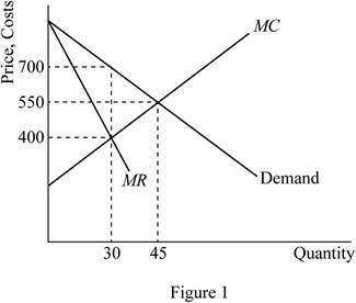
Figure 1 represents the marginal-revenue, marginal-cost, and demand curves. The horizontal axis represents the quantity and the vertical axis the prices, revenues and costs. The MR and MC curves cross between quantities of 400,000 and 500,000 which signify that the firm is maximizing profit in that region.
Concept introduction:
Marginal product of labor (MPL): Marginal product of labor refers to the additional output produced due to employing one more unit of labor.
Marginal product of capital (MPC): Marginal product of capital refers to the additional output produced due to employing one more unit of capital.
Profit maximization: A firm can maximize its profit at the point where its marginal revenue is equal to marginal cost.
Subpart (d):
Deadweight loss.
Subpart (d):
Explanation of Solution
The deadweight loss is depicted by area DWL in figure 1. Deadweight loss is greater in
Concept introduction:
Deadweight loss: Deadweight loss refers to loss of total economic benefit that arises due to the inefficient allocation of resource.
Subpart (e):
Change in profit.
Subpart (e):
Explanation of Solution
The price would not change if the author were paid $3 million instead of $2 million, the publisher since there would be no change in marginal cost or marginal revenue. The result would be a fall in the firm’s profit.
Concept introduction:
Profit: Profit refers to the excess revenue after subtracting the total cost from the total revenue.
Subpart (f):
Maximize economic efficiency.
Subpart (f):
Explanation of Solution
To maximize economic efficiency, the publisher would charge the price at $10 per book. This is because it is the marginal cost of the book. At price $10 per book, the publisher would receive negative profits equal to the amount paid to the author.
Concept introduction:
Economic efficiency: Economic efficiency is the situation where the economy is efficient. Which means that the marginal benefit from the last unit produced is equal to the marginal cost of production and the economic surplus will be at maximum.
Want to see more full solutions like this?
Chapter 15 Solutions
Bundle: Principles of Microeconomics, 7th + LMS Integrated Aplia, 1 term Printed Access Card

- You are the manager of a large automobile dealership who wants to learn more about the effective- ness of various discounts offered to customers over the past 14 months. Following are the average negotiated prices for each month and the quantities sold of a basic model (adjusted for various options) over this period of time. 1. Graph this information on a scatter plot. Estimate the demand equation. What do the regression results indicate about the desirability of discounting the price? Explain. Month Price Quantity Jan. 12,500 15 Feb. 12,200 17 Mar. 11,900 16 Apr. 12,000 18 May 11,800 20 June 12,500 18 July 11,700 22 Aug. 12,100 15 Sept. 11,400 22 Oct. 11,400 25 Nov. 11,200 24 Dec. 11,000 30 Jan. 10,800 25 Feb. 10,000 28 2. What other factors besides price might be included in this equation? Do you foresee any difficulty in obtaining these additional data or incorporating them in the regression analysis?arrow_forwardsimple steps on how it should look like on excelarrow_forwardConsider options on a stock that does not pay dividends.The stock price is $100 per share, and the risk-free interest rate is 10%.Thestock moves randomly with u=1.25and d=1/u Use Excel to calculate the premium of a10-year call with a strike of $100.arrow_forward
- Please solve this, no words or explanations.arrow_forward17. Given that C=$700+0.8Y, I=$300, G=$600, what is Y if Y=C+I+G?arrow_forwardUse the Feynman technique throughout. Assume that you’re explaining the answer to someone who doesn’t know the topic at all. Write explanation in paragraphs and if you use currency use USD currency: 10. What is the mechanism or process that allows the expenditure multiplier to “work” in theKeynesian Cross Model? Explain and show both mathematically and graphically. What isthe underpinning assumption for the process to transpire?arrow_forward
- Use the Feynman technique throughout. Assume that you’reexplaining the answer to someone who doesn’t know the topic at all. Write it all in paragraphs: 2. Give an overview of the equation of exchange (EoE) as used by Classical Theory. Now,carefully explain each variable in the EoE. What is meant by the “quantity theory of money”and how is it different from or the same as the equation of exchange?arrow_forwardZbsbwhjw8272:shbwhahwh Zbsbwhjw8272:shbwhahwh Zbsbwhjw8272:shbwhahwhZbsbwhjw8272:shbwhahwhZbsbwhjw8272:shbwhahwharrow_forwardUse the Feynman technique throughout. Assume that you’re explaining the answer to someone who doesn’t know the topic at all:arrow_forward
 Essentials of Economics (MindTap Course List)EconomicsISBN:9781337091992Author:N. Gregory MankiwPublisher:Cengage Learning
 Microeconomics: Private and Public Choice (MindTa...EconomicsISBN:9781305506893Author:James D. Gwartney, Richard L. Stroup, Russell S. Sobel, David A. MacphersonPublisher:Cengage Learning
 Economics: Private and Public Choice (MindTap Cou...EconomicsISBN:9781305506725Author:James D. Gwartney, Richard L. Stroup, Russell S. Sobel, David A. MacphersonPublisher:Cengage Learning
 Principles of Economics 2eEconomicsISBN:9781947172364Author:Steven A. Greenlaw; David ShapiroPublisher:OpenStax
 Managerial Economics: Applications, Strategies an...EconomicsISBN:9781305506381Author:James R. McGuigan, R. Charles Moyer, Frederick H.deB. HarrisPublisher:Cengage Learning