Chapter 15, Problem 17CP

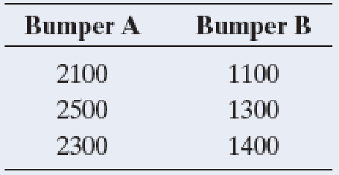
Car bumper damage An automobile company compares two types of front bumper for its new model by driving sample cars into a concrete wall at 15 miles per hour. The response is the amount of damage to the car, as measured by the repair costs, in dollars. Due to the costs, the study uses only six cars, obtaining results for three bumpers of each type. The results are in the table.

1. a. Find the ranks and the mean rank for each bumper type.
2. b. Show that there are 20 possible allocations of ranks to the two bumper types.
3. c. Explain why the observed ranks for the two groups are one of the two most extreme ways the two groups can differ, for the 20 possible allocations of the ranks.
4. d. Explain why the P-value for the two-sided test equals 0.10.

To determine

Find the ranks of the two groups of Bumper.

Find the mean ranks of the two groups of Bumper.

Answer to Problem 17CP

The ranks for each Bumper type are given below:

Ranks of Bumper-A	Ranks of Bumper-B
4	1
5	2
6	3

The mean ranks for each bumper type are given below:

Group	Sum
Bumper-A	$\frac{15}{3}=5$
Bumper-B	$\frac{6}{3}=2$

Explanation of Solution

The data represent the repair costs of Bumper A type cars and Bumper B type cars in dollars. Due to Financial crisis only 6 cars are considered for the study.

The results are as follows:

Bumper A: 2,100, 2,500, 2,300.

Bumper B: 1,100, 1,300, 1,400.

Here, it is given that cars were ranked from 1 to 6, where 1 represents the less repair cost.

The ranks for the two groups are obtained as given below:

Step-1: Arrange the data in ascending order as follows:

1,100, 1,300, 1,400, 2,100, 2,300, 2,500.

Step-2: Rank all the ordered values from 1 to 6. Here, the repair costs are ranked from 1, where 1 represents the lowest repair cost (Best quality car).

Step-3: Identify the values of Bumper-A and Bumper-B and then divide the ranks based on the corresponding values of two groups.

The ranks for each Bumper type are given below:

Ranks of Bumper-A	Ranks of Bumper-B
4	1
5	2
6	3

The mean ranks for each bumper type are given below:

Group	Sum
Bumper-A	$\frac{15}{3}=5$
Bumper-B	$\frac{6}{3}=2$

To determine

Find all the possible ways the ranks could be allocated to each of the Bumper type with no ties.

Answer to Problem 17CP

All the possible ways the ranks could be allocated to each of the Bumper type with no ties are given below:

S no	Ranks of Bumper-A	Ranks of Bumper-B
1	(1,2,3)	(4,5,6)
2	(1,2,4)	(3,5,6)
3	(1,2,5)	(3,4,6)
4	(1,2,6)	(3,4,5)
5	(1,3,4)	(2,5,6)
6	(1,3,5)	(2,4,6)
7	(1,3,6)	(2,4,5)
8	(1,4,5)	(2,3,6)
9	(1,4,6)	(2,3,5)
10	(1,5,6)	(2,3,4)
11	(2,3,4)	(1,5,6)
12	(2,3,5)	(1,4,6)
13	(2,3,6)	(1,4,5)
14	(2,4,5)	(1,3,6)
15	(2,4,6)	(1,3,5)
16	(2,5,6)	(1,3,4)
17	(3,4,5)	(1,2,6)
18	(3,4,6)	(1,2,5)
19	(3,5,6)	(1,2,4)
20	(4,5,6)	(1,2,3)

Explanation of Solution

Each possible outcome divides the ranks of 1, 2, 3, 4, 5, 6 into two groups. Three ranks are given to the group Bumper A and three ranks are given to the group Bumper B.

The possible rankings are shown in the below table:

S no	Ranks of Bumper-A	Ranks of Bumper-B
1	(1,2,3)	(4,5,6)
2	(1,2,4)	(3,5,6)
3	(1,2,5)	(3,4,6)
4	(1,2,6)	(3,4,5)
5	(1,3,4)	(2,5,6)
6	(1,3,5)	(2,4,6)
7	(1,3,6)	(2,4,5)
8	(1,4,5)	(2,3,6)
9	(1,4,6)	(2,3,5)
10	(1,5,6)	(2,3,4)
11	(2,3,4)	(1,5,6)
12	(2,3,5)	(1,4,6)
13	(2,3,6)	(1,4,5)
14	(2,4,5)	(1,3,6)
15	(2,4,6)	(1,3,5)
16	(2,5,6)	(1,3,4)
17	(3,4,5)	(1,2,6)
18	(3,4,6)	(1,2,5)
19	(3,5,6)	(1,2,4)
20	(4,5,6)	(1,2,3)

To determine

Explain the reason behind the given claim.

Explanation of Solution

The given claim is: The observed ranks for the two Bumper types are one of the two extreme ways in which the two Bumper types can differ.

The claim states that, the ranks of two Bumper types should differ extremely. In other words, it can be said that, Bumper-A and Bumper-B should have extreme ranks.

Part(b) gives the, 20 possible ways the ranks could be allocated to each of the Bumper type with no ties.

From the 20 possible ranks, there are 2 ways in which the ranks are extreme.

The two ways in which the allocation of ranks is extreme are given:

S no	Ranks of Bumper-A	Ranks of Bumper-B
1	(1,2,3)	(4,5,6)
2	(4,5,6)	(1,2,3)

Since, out of 20 possible ways there are only 2 ways in which the ranks are extreme, it is said that the observed ranks for the two Bumper types are one of the two extreme ways in which the two Bumper types can differ.

To determine

Explain the reason behind $\text{P-value=0}\text{.10}$ for two sided hypothesis test.

Explanation of Solution

Calculation:

The hypotheses are given below:

Null hypothesis:

$H_0:$ The two Bumper types are identical in quality.

Alternative hypothesis:

$H_a:$ The quality of two Bumper types have differs.

Here, the alternative hypothesis is two sided. It represents that the mean rank in population of cars assigned to Bumper-A is not equal to the mean rank in population of cars assigned to Bumper-B.

Here, it is given that observed ranks for the two Bumper types are one of the two extreme ways in which the two Bumper types can differ.

The P-value is the probability that the ranks of Bumper types are extreme.

It is known that, out of 20 possible ways, there are only two ways in which the Bumper ranks are extreme.

The P-value is obtained as given below:

$\begin{array}{c}\text{P-value}=\frac{2}{20}\\ \text{=0}\text{.10}\end{array}$

Therefore, the P–value is 0.1.