Subpart (a):
Profit maximization.
Subpart (a):
Explanation of Solution
Table – 1 represents the value of quantity, total cost, and total revenue.
Table – 1
| Quantity | Total cost | Total revenue |
| 0 | 8 | 0 |
| 1 | 9 | 8 |
| 2 | 10 | 16 |
| 3 | 11 | 24 |
| 4 | 13 | 32 |
| 5 | 19 | 40 |
| 6 | 27 | 48 |
| 7 | 37 | 56 |
The profit can be calculated by using the following formula:
Substitute the respective value in equation (1) and calculate the profit.
The profit is –$8.
Table – 2 shows the value of the profit that is obtained, by using equation (1).
Table – 2
| Quantity | Total cost | Total revenue | Profit |
| 0 | 8 | 0 | –8 |
| 1 | 9 | 8 | –1 |
| 2 | 10 | 16 | 6 |
| 3 | 11 | 24 | 13 |
| 4 | 13 | 32 | 19 |
| 5 | 19 | 40 | 21 |
| 6 | 27 | 48 | 21 |
| 7 | 37 | 56 | 19 |
From the above table, the firm can maximize profit when they produce five or six units of output.
Concept introduction:
Perfect competitive firm:
Marginal Revenue (MR): Marginal revenue refers to the additional revenue earned due to increasing one more unit of output.
Marginal Cost (MC): The marginal cost refers to the amount of an additional cost incurred in the process of increasing one more unit of output.
Subpart (b):
Profit maximization.
Subpart (b):
Explanation of Solution
The marginal revenue can be calculated by using the following formula:
Substitute the respective value in equation (2) and calculate marginal revenue.
The marginal revenue is $8.
Table – 3 shows the value of the marginal revenue that obtained by using equation (2).
Table – 3
| Quantity | Total cost | Total revenue | Marginal revenue | Profit |
| 0 | 8 | 0 | – | –8 |
| 1 | 9 | 8 | 8 | –1 |
| 2 | 10 | 16 | 8 | 6 |
| 3 | 11 | 24 | 8 | 13 |
| 4 | 13 | 32 | 8 | 19 |
| 5 | 19 | 40 | 8 | 21 |
| 6 | 27 | 48 | 8 | 21 |
| 7 | 37 | 56 | 8 | 19 |
The marginal cost can be calculated by using the following formula:
Substitute the respective value in equation (3) and calculate the marginal cost.
The marginal cost is $8.
Table – 4 shows the value of the marginal cost that is obtained by using equation (3).
Table – 4
| Quantity | Total cost | Marginal cost | Total revenue | Marginal revenue | Profit |
| 0 | 8 | – | 0 | – | –8 |
| 1 | 9 | 1 | 8 | 8 | –1 |
| 2 | 10 | 1 | 16 | 8 | 6 |
| 3 | 11 | 1 | 24 | 8 | 13 |
| 4 | 13 | 2 | 32 | 8 | 19 |
| 5 | 19 | 6 | 40 | 8 | 21 |
| 6 | 27 | 8 | 48 | 8 | 21 |
| 7 | 37 | 10 | 56 | 8 | 19 |
Figure – 1 shows the marginal revenue curve and marginal cost curve.
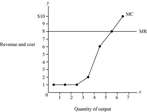
Figure – 1
From the above figure, the x axis shows the quantity of output and the y axis shows the price, that is, revenue and cost. From the above figure, the intersecting point shows the point the firm’s maximizing profit when they produce five or six units of output.
Concept introduction:
Perfect competitive firm: Perfect competition refers to the market structure featuring more number of sellers and buyers in the market, where the firm can sell homogenous products.
Marginal Revenue (MR): Marginal revenue refers to the additional revenue earned due to increasing one more unit of output.
Marginal Cost (MC): The marginal cost refers to the amount of an additional cost incurred in the process of increasing one more unit of output.
Subpart (c):
Profit in the long run.
Subpart (c):
Explanation of Solution
Since the marginal revenue is the same as each level of the quantity, the firm is in a competitive industry. The firm is earning an economic profit. Generally, firms in the long run earn a normal profit. Thus, the firm is not in the long run equilibrium.
Concept introduction:
Long run: Thelong run refers to the time, which changes the production variable to adjust to the market situation.
Want to see more full solutions like this?
Chapter 14 Solutions
Bundle: Principles of Microeconomics, 7th + LMS Integrated Aplia, 1 term Printed Access Card

- Can you please help with this one. Some economists argue that taxing consumption is more efficient than taxing income. Following the same argument, the minister of finance of a country introduced a new tax for sugar based products “sugar tax” to promote healthy eating in the economy. Please use relevant diagrams to explain the impact of the tax on consumers, producers and the tax revenue when sugar is elastic and inelastic.arrow_forwardprofit maximizing and loss minamization fire dragon co mindtaparrow_forwardProblem 3 You are given the following demand for European luxury automobiles: Q=1,000 P-0.5.2/1.6 where P-Price of European luxury cars PA = Price of American luxury cars P, Price of Japanese luxury cars I= Annual income of car buyers Assume that each of the coefficients is statistically significant (i.e., that they passed the t-test). On the basis of the information given, answer the following questions 1. Comment on the degree of substitutability between European and American luxury cars and between European and Japanese luxury cars. Explain some possible reasons for the results in the equation. 2. Comment on the coefficient for the income variable. Is this result what you would expect? Explain. 3. Comment on the coefficient of the European car price variable. Is that what you would expect? Explain.arrow_forward
- Problem 2: A manufacturer of computer workstations gathered average monthly sales figures from its 56 branch offices and dealerships across the country and estimated the following demand for its product: Q=+15,000-2.80P+150A+0.3P+0.35Pm+0.2Pc (5,234) (1.29) (175) (0.12) (0.17) (0.13) R²=0.68 SER 786 F=21.25 The variables and their assumed values are P = Price of basic model = 7,000 Q==Quantity A = Advertising expenditures (in thousands) = 52 P = Average price of a personal computer = 4,000 P. Average price of a minicomputer = 15,000 Pe Average price of a leading competitor's workstation = 8,000 1. Compute the elasticities for each variable. On this basis, discuss the relative impact that each variable has on the demand. What implications do these results have for the firm's marketing and pricing policies? 2. Conduct a t-test for the statistical significance of each variable. In each case, state whether a one-tail or two-tail test is required. What difference, if any, does it make to…arrow_forwardYou are the manager of a large automobile dealership who wants to learn more about the effective- ness of various discounts offered to customers over the past 14 months. Following are the average negotiated prices for each month and the quantities sold of a basic model (adjusted for various options) over this period of time. 1. Graph this information on a scatter plot. Estimate the demand equation. What do the regression results indicate about the desirability of discounting the price? Explain. Month Price Quantity Jan. 12,500 15 Feb. 12,200 17 Mar. 11,900 16 Apr. 12,000 18 May 11,800 20 June 12,500 18 July 11,700 22 Aug. 12,100 15 Sept. 11,400 22 Oct. 11,400 25 Nov. 11,200 24 Dec. 11,000 30 Jan. 10,800 25 Feb. 10,000 28 2. What other factors besides price might be included in this equation? Do you foresee any difficulty in obtaining these additional data or incorporating them in the regression analysis?arrow_forwardsimple steps on how it should look like on excelarrow_forward
- Consider options on a stock that does not pay dividends.The stock price is $100 per share, and the risk-free interest rate is 10%.Thestock moves randomly with u=1.25and d=1/u Use Excel to calculate the premium of a10-year call with a strike of $100.arrow_forwardCompute the Fourier sine and cosine transforms of f(x) = e.arrow_forwardDon't use ai to answer I will report you answerarrow_forward
 Essentials of Economics (MindTap Course List)EconomicsISBN:9781337091992Author:N. Gregory MankiwPublisher:Cengage Learning
 Microeconomics: Principles & PolicyEconomicsISBN:9781337794992Author:William J. Baumol, Alan S. Blinder, John L. SolowPublisher:Cengage Learning

 Principles of Economics (MindTap Course List)EconomicsISBN:9781305585126Author:N. Gregory MankiwPublisher:Cengage Learning
 Principles of Economics, 7th Edition (MindTap Cou...EconomicsISBN:9781285165875Author:N. Gregory MankiwPublisher:Cengage Learning