Chapter 14, Problem 22CAP

(a)

To determine

Complete the F table.

Determine whether decision to retain or rejectthe null hypothesis for each hypothesis test.

Answer to Problem 22CAP

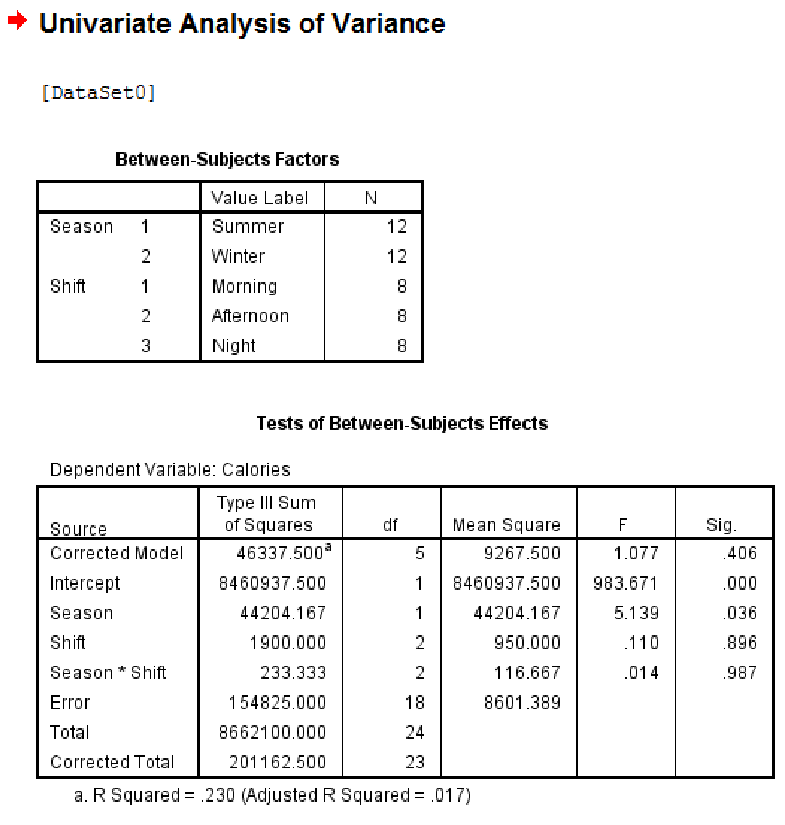
The completedF table is,

Source of Variation	SS	df	MS	$F_{\text{obt}}$
Season	44,204.17	1	44,204.17	5.139
Shift	1,900.00	2	950.00	0.110
Season $\times$ Shift	233.34	2	116.67	0.014
Error	154,825.00	18	8,601.39
Total	201,162.51	23

The decision is to reject the null hypothesis for Season, the group means for main effect Season (summer, winter) do significantly vary in the population.

The decision is to retain the null hypothesis for shift, the group means for main effect shift (morning, afternoon, evening) do not significantly vary in the population.

The decision is to retainthe null hypothesis for interaction effect; the means of season do not significantly vary by shift or the combinations of these factors.

Explanation of Solution

Calculation:

From the information given that, the study is based on the eating patterns that might contribute toobesity and these measures the average number of calories (permeal) consumed by shift workers (morning, afternoon, night)during two seasons (summer and winter).

Software procedure:

Step by step procedure to obtain the Two-way between-subjects ANOVA using SPSS software is given as,

• Choose Variable view.
• Under the name, enter the names as Season, Shift andCalories.
• Choose Data view, enter the data for as Season, Shift andCalories, respectively.
• Choose Analyze>General Linear Model>Univariate.
• Enter calories in Dependent variable dialog box.
• Send as Season, Shift into Fixed factors.
• Click on Options button.
• Send Season, Shift into Display Means for dialog box.
• Click on Continue button.
• Click OK.

Output using SPSS software is given below:

The completed F table is,

Source of Variation	SS	df	MS	$F_{\text{obt}}$
Season	44,204.17	1	44,204.17	5.139
Shift	1,900.00	2	950.00	0.110
Season $\times$ Shift	233.34	2	116.67	0.014
Error	154,825.00	18	8,601.39
Total	201,162.51	23

Decision rules:

• If the test statistic value is greater than the critical value, then reject the null hypothesis
• If the test statistic value is smaller than the critical value, then retain the null hypothesis

Hypothesis test for main effect factor A (Season):

Let ${\sigma }_{\mu \text{'}s}^2$ be the group means of the main effect Season.

Null hypothesis:

$H_0:{\sigma }_{\mu \text{'}s}^2=0$

That is, the group means for main effect Season (summer, winter) do not significantly vary in the population.

Alternative hypothesis:

$H_0:{\sigma }_{\mu \text{'}s}^2>0$

That is, the group means for main effect Season (summer, winter)  do significantly vary in the population.

Critical value:

The considered significance level is $\alpha =0.05$.

The degrees of freedom for numerator are 1, the degrees of freedom for denominator are 18 from completed F table.

From the Appendix B: Table B.3-Critical values for F distribution:

• Locate the value 1 in degrees of freedom numerator row.
• Locate the value 18 in degrees of freedom denominator row.
• Locate the 0.05 level of significance (value in lightface type) in combined row.
• The intersecting value that corresponds to the (1, 18) with level of significance 0.05 is 4.41.

Thus, the critical value for $df=\left(1,18\right)$ with 0.05, level of significance is 4.41.

Conclusion:

The value of test statistic is 5.139.

The critical value is 4.41.

The test statistic value is greater than the critical value.

The test statistic value falls under critical region.

Hence the null hypothesis is rejected.

The decision is the group means for main effect Season (summer, winter) do significantly vary in the population.

Hypothesis test for main effect factor B (Shift):

Let ${\sigma }_{\mu \text{'}s}^2$ be the group means of the main effect shift.

Null hypothesis:

$H_0:{\sigma }_{\mu \text{'}s}^2=0$

That is, the group means for main effect shift (morning, afternoon, evening) do not significantly vary in the population.

Alternative hypothesis:

$H_0:{\sigma }_{\mu \text{'}s}^2>0$

That is, the group means for main effect shift (morning, afternoon, evening) do significantly vary in the population.

Critical value:

The considered significance level is $\alpha =0.05$.

The degrees of freedom for numerator are 2, the degrees of freedom for denominator are 18 from completed F table.

From the Appendix B: Table B.3-Critical values for F distribution:

• Locate the value 2 in degrees of freedom numerator row.
• Locate the value 18 in degrees of freedom denominator row.
• Locate the 0.05 level of significance (value in lightface type) in combined row.
• The intersecting value that corresponds to the (2, 18) with level of significance 0.05 is 3.55.

Thus, the critical value for $df=\left(2,18\right)$ with 0.05, level of significance is 3.55.

Conclusion:

The value of test statistic is 0.110.

The critical value is 3.55.

The test statistic value is less than the critical value.

The test statistic value does not falls under critical region.

Hence the null hypothesis is retained.

The decision is the group means for main effect shift (morning, afternoon, evening) do significantly vary in the population.

Hypothesis test for interaction effect of factor A and B:

Let ${\sigma }_{\mu \text{'}s}^2$ be the group means of the interaction effect.

Null hypothesis:

$H_0:{\sigma }_{\mu \text{'}s}^2=0$

That is, the means of season do not significantly vary by shift or the combinations of these factors.

Alternative hypothesis:

$H_0:{\sigma }_{\mu \text{'}s}^2>0$

That is, the means of season do significantly vary by shift or the combinations of these factors.

Critical value:

The considered significance level is $\alpha =0.05$. The degrees of freedom for numerator are 2, the degrees of freedom for denominator are 18 from completed F table.From the Appendix B: Table B.3-Critical values for F distribution the critical value is 3.55.

Thus, the critical value for $df=\left(2,18\right)$ with 0.05, level of significance is 3.55.

Conclusion:

The value of test statistic is 0.014.

The critical value is 3.55.

The test statistic value is less than the critical value.

The test statistic value does not falls under critical region.

Hence the null hypothesis is retained.

The decision is the means of season do not significantly vary by shift or the combinations of these factors.

2.

To determine

Explain why the tests of post hoc are not necessary.

Answer to Problem 22CAP

The tests of post hoc are not necessary for this test because only the main effect ‘season’ is significant and another main effect ‘shift’ is not significant.

Explanation of Solution

Justification: The post hoc tests are conducted only when the two main effects in the study are significant. The result of the study is that the main effect ‘season’ is significant this effect has only two levels, but another main effect ‘shift’ is not significant and also the interaction effect bewteen both the factors is not significant. This shows that, conducting post hoc tests is not necessary since the main effect ‘shift’ is not significant.