Subpart (a):
Revenues, costs and profits.
Subpart (a):
Explanation of Solution
Table -1 shows the total quantity and respective
Table -1
| Price | Quantity |
| 100 | 0 |
| 90 | 100,000 |
| 80 | 200,000 |
| 70 | 300,000 |
| 60 | 400,000 |
| 50 | 500,000 |
| 40 | 600,000 |
| 30 | 700,000 |
| 20 | 800,000 |
| 10 | 900,000 |
| 0 | 1,000,000 |
Total revenue can be calculated by using the following formula.
Substitute the respective values in Equation (1) to calculate the total revenue at price $90.
Total revenue is $9,000,000.
Total cost can be calculated by using the following formula.
Substitute the respective values in Equation (2) to calculate the total cost at quantity 100,000 units.
Total cost is $2,000,000.
Profit can be calculated by using the following formula.
Substitute the respective values in Equation (3) to calculate the profit for the quantity 100,000 units.
Profit is 7,000,000.
Table -2 shows the total revenue, total cost and profit that are obtained by using Equations (1), (2) and (3).
Table -2
| Price | Quantity | Total revenue | Total cost | Profit |
| 100 | 0 | 0 | 2,000,000 | -2,000,000 |
| 90 | 100,000 | 9,000,000 | 3,000,000 | 6,000,000 |
| 80 | 200,000 | 16,000,000 | 4,000,000 | 12,000,000 |
| 70 | 300,000 | 21,000,000 | 5,000,000 | 16,000,000 |
| 60 | 400,000 | 24,000,000 | 6,000,000 | 18,000,000 |
| 50 | 500,000 | 25,000,000 | 7,000,000 | 18,000,000 |
| 40 | 600,000 | 24,000,000 | 8,000,000 | 16,000,000 |
| 30 | 700,000 | 21,000,000 | 9,000,000 | 12,000,000 |
| 20 | 800,000 | 16,000,000 | 10,000,000 | 6,000,000 |
| 10 | 900,000 | 9,000,000 | 11,000,000 | -2,000,000 |
| 0 | 1,000,000 | 0 | 12,000,000 | -12,000,000 |
The maximum profit of $18 million is obtained at a quantity of 500,000 at a price of $50. Thus, the
Concept introduction:
Profit: Profit refers to the excess revenue after subtracting the total cost from the total revenue.
Total revenue: Total revenue refers to the revenue of a firm through its total sale of goods.
Total cost: Total cost refers to the cost of all the inputs used by the firm. It includes both the fixed cost and the variable costs.
Subpart (b):
Calculate marginal revenue.
Subpart (b):
Explanation of Solution
Marginal revenue can be calculated as follows:
Substitute the respective values in equation (4) to calculate the marginal revenue at price level $60.
Marginal revenue is $30.
Table -3 shows the marginal revenue that obtained by using equation (4).
Table -3
| Price | Quantity | Total revenue | Marginal revenue |
| 100 | 0 | 0 | - |
| 90 | 100,000 | 9,000,000 | $90 |
| 80 | 200,000 | 16,000,000 | 70 |
| 70 | 300,000 | 21,000,000 | 50 |
| 60 | 400,000 | 24,000,000 | 30 |
| 50 | 500,000 | 25,000,000 | 10 |
| 40 | 600,000 | 24,000,000 | -10 |
| 30 | 700,000 | 21,000,000 | -30 |
| 20 | 800,000 | 16,000,000 | -50 |
| 10 | 900,000 | 9,000,000 | -70 |
| 0 | 1,000,000 | 0 | -90 |
From table 4, it can be inferred that Marginal Revenue is less than price. Since the demand curve slopes downwards, Price declines when quantity rises. The marginal revenue declines even more than price because the firm loses revenue on all the units of the good sold when it lowers the price.
Concept introduction:
Marginal revenue: Marginal revenue refers to the amount of extra revenue attained in the process of increasing one more unit of output.
Subpart (c):
Profit maximization.
Subpart (c):
Explanation of Solution
Figure 1illustrates the
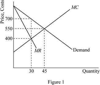
Figure 1 represents the marginal-revenue, marginal-cost, and demand curves. The horizontal axis represents the quantity and the vertical axis the prices, revenues and costs. The MR and MC curves cross between quantities of 400,000 and 500,000 which signify that the firm is maximizing profit in that region.
Concept introduction:
Marginal product of labor (MPL): Marginal product of labor refers to the additional output produced due to employing one more unit of labor.
Marginal product of capital (MPC): Marginal product of capital refers to the additional output produced due to employing one more unit of capital.
Profit maximization: A firm can maximize its profit at the point where its marginal revenue is equal to marginal cost.
Subpart (d):
Deadweight loss.
Subpart (d):
Explanation of Solution
The deadweight loss is depicted by area DWL in figure 1. Deadweight loss is greater in
Concept introduction:
Deadweight loss: Deadweight loss refers to loss of total economic benefit that arises due to the inefficient allocation of resource.
Subpart (e):
Change in profit.
Subpart (e):
Explanation of Solution
The price would not change if the author were paid $3 million instead of $2 million, the publisher since there would be no change in marginal cost or marginal revenue. The result would be a fall in the firm’s profit.
Concept introduction:
Profit: Profit refers to the excess revenue after subtracting the total cost from the total revenue.
Subpart (f):
Maximize economic efficiency.
Subpart (f):
Explanation of Solution
To maximize economic efficiency, the publisher would charge the price at $10 per book. This is because it is the marginal cost of the book. At price $10 per book, the publisher would receive negative profits equal to the amount paid to the author.
Concept introduction:
Economic efficiency: Economic efficiency is the situation where the economy is efficient. Which means that the marginal benefit from the last unit produced is equal to the marginal cost of production and the economic surplus will be at maximum.
Want to see more full solutions like this?
Chapter 14 Solutions
Bundle: Essentials Of Economics, Loose-leaf Version, 8th + Lms Integrated Mindtap Economics, 1 Term (6 Months) Printed Access Card

- agrody calming Inted 001 and me 2. A homeowner is concerned about the various air pollutants (e.g., benzene and methane) released in her house when she cooks with natural gas. She is considering replacing her gas oven and stove with an electric stove comprising an induction cooktop and convection oven. The new appliance costs $900 to purchase and install. Capping the old gas line costs an additional $150 (a one-time fee). The old line must be inspected for leaks each year after capping, at a cost of $35 for each inspection. a. If the homeowner plans to remain in the house for four more years and the discount rate is 4%, what is the minimum present value of the benefits that the homeowner would need to experience for this purchase to be justified based on its private net sub present value? b. While trying to understand how she might express the value of reduced exposure to indoor air pollutants in dollar terms, the homeowner consulted the EPA website and found estimates provided by…arrow_forwardAfter the ban is imposed, Joe’s firm switches to the more expensive biodegradable disposable cups. This increases the cost associated with each cup of coffee it produces. Which cost curve(s) will be impacted by the use of the more expensive biodegradable disposable cups? Why? Which cost curve(s) will not shift, and why not? Please use the table below to answer this question. For the second column (“Impacted? If so, how?”), please use one of the following three choices: No shift; Shifts up (i.e., increases: at nearly any given quantity, the cost goes up); or Shifts down (i.e., decreases: at nearly any given quantity, the cost goes down). $ Cost Curve Impacted? If so, how? Explanation of the Shift: Why or Why Not AFC No shift. Fix costs stay the same, regardless of quantity. Fixed cost is calculated as Fixed Cost/Quantity. Since fixed costs remain unchanged, AFC stays the same for each quantity. MC Shifts up. Since the biodegradable cups are more expensive, the…arrow_forwardStyrofoam is non-biodegradable and is not easily recyclable. Many cities and at least one state have enacted laws that ban the use of polystyrene containers. These locales understand that banning these containers will force many businesses to turn to other more expensive forms of packaging and cups, but argue the ban is environmentally important. Shane owns a firm with a conventional production function resulting in U-shaped ATC, AVC, and MC curves. Shane's business sells takeout food and drinks that are currently packaged in styrofoam containers and cups. Graph the short-run AFC0, AVC0, ATC0, and MC0 curves for Shane's firm before the ban on using styrofoam containers.arrow_forward
- PART II: Multipart Problems wood or solem of triflussd aidi 1. Assume that a society has a polluting industry comprising two firms, where the industry-level marginal abatement cost curve is given by: MAC = 24 - ()E and the marginal damage function is given by: MDF = 2E. What is the efficient level of emissions? b. What constant per-unit emissions tax could achieve the efficient emissions level? points) c. What is the net benefit to society of moving from the unregulated emissions level to the efficient level? In response to industry complaints about the costs of the tax, a cap-and-trade program is proposed. The marginal abatement cost curves for the two firms are given by: MAC=24-E and MAC2 = 24-2E2. d. How could a cap-and-trade program that achieves the same level of emissions as the tax be designed to reduce the costs of regulation to the two firms?arrow_forwardOnly #4 please, Use a graph please if needed to help provearrow_forwarda-carrow_forward
- For these questions, you must state "true," "false," or "uncertain" and argue your case (roughly 3 to 5 sentences). When appropriate, the use of graphs will make for stronger answers. Credit will depend entirely on the quality of your explanation. 1. If the industry facing regulation for its pollutant emissions has a lot of political capital, direct regulatory intervention will be more viable than an emissions tax to address this market failure. 2. A stated-preference method will provide a measure of the value of Komodo dragons that is more accurate than the value estimated through application of the travel cost model to visitation data for Komodo National Park in Indonesia. 3. A correlation between community demographics and the present location of polluting facilities is sufficient to claim a violation of distributive justice. olsvrc Q 4. When the damages from pollution are uncertain, a price-based mechanism is best equipped to manage the costs of the regulator's imperfect…arrow_forwardFor environmental economics, question number 2 only please-- thank you!arrow_forwardFor these questions, you must state "true," "false," or "uncertain" and argue your case (roughly 3 to 5 sentences). When appropriate, the use of graphs will make for stronger answers. Credit will depend entirely on the quality of your explanation. 1. If the industry facing regulation for its pollutant emissions has a lot of political capital, direct regulatory intervention will be more viable than an emissions tax to address this market failure. cullog iba linevoz ve bubivorearrow_forward
 Essentials of Economics (MindTap Course List)EconomicsISBN:9781337091992Author:N. Gregory MankiwPublisher:Cengage Learning
 Microeconomics: Private and Public Choice (MindTa...EconomicsISBN:9781305506893Author:James D. Gwartney, Richard L. Stroup, Russell S. Sobel, David A. MacphersonPublisher:Cengage Learning
 Economics: Private and Public Choice (MindTap Cou...EconomicsISBN:9781305506725Author:James D. Gwartney, Richard L. Stroup, Russell S. Sobel, David A. MacphersonPublisher:Cengage Learning
 Principles of Economics 2eEconomicsISBN:9781947172364Author:Steven A. Greenlaw; David ShapiroPublisher:OpenStax
 Managerial Economics: Applications, Strategies an...EconomicsISBN:9781305506381Author:James R. McGuigan, R. Charles Moyer, Frederick H.deB. HarrisPublisher:Cengage Learning