Videos
a.
Test whether the data suggests a linear relationship between specific gravity and at least one of the predictors at 1% level of significance.
a.
Answer to Problem 56E
There is sufficient evidence to conclude that the there is a use of linear relationship between specific gravity and at least one of the five predictors number of fibers in springwood, number of fibers in summerwood, percentage of springwood, light absorption in springwood and light absorption in summerwood at 1% level of significance.
Explanation of Solution
Given info:
A sample of 20 mature woods were taken and the number of fibers in springwood, number of fibers in summerwood, percentage of springwood, light absorption in springwood and light absorption in summerwood were noted .
The coefficient of determination
Calculation:
The test hypotheses are given below:
Null hypothesis:
That is, there is no use of linear relationship between specific gravity and the five predictors.
Alternative hypothesis:
That is, there is a use of linear relationship between specific gravity and at least one of the five predictors.
Test statistic:
Substitute
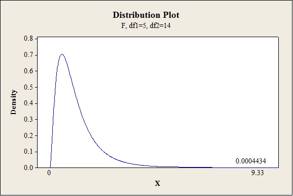
P-value:
Software procedure:
- Click on Graph, select View Probability and click OK.
- Select F, enter 5 in numerator df and 14 in denominator df.
- Under Shaded Area Tab select X value under Define Shaded Area By and select Right tail.
- Choose X value as 9.33.
- Click OK.
Output obtained from MINITAB is given below:
Conclusion:
The P-value is 0.000 and the level of significance is 0.01.
The P-value is lesser than the level of significance.
That is
Thus, the null hypothesis is rejected.
Hence, there is sufficient evidence to conclude that there is ause of linear relationship between specific gravity and at least one of the five predictors at 1% level of significance.
b.
Calculate the adjusted
b.
Answer to Problem 56E
The adjusted
The adjusted
Explanation of Solution
Given info:
The
Calculation:
Adjusted
Adjusted
Substitute n as 20,k as 5,
Thus, the adjusted
Adjusted
Substitute n as 20, k as 4,
Thus, the adjusted
c.
Identify whether the data suggests that variables
Test the hypothesis to see whether the variables
c.
Answer to Problem 56E
Yes, the data suggests that variables
There issufficient evidence to conclude the variables
Explanation of Solution
Given info:
The
Calculation:
After dropping the three variables
The test hypotheses are given below:
Null hypothesis:
That is, there is no use of linear relationship betweenspecific gravity and at least one of the predictors, percentage of springwood and light absorption in summerwood.
Alternative hypothesis:
That is, there is use of linear relationship between specific gravity and at least one of the predictors, percentage of springwood and light absorption in summerwood.
From the
Similarly, the sum of squares due to error for the reduced model
Test statistic:
Where,
n represents the total number of observations.
k represents the number of predictors on the full model.
l represents the number of predictors on the reduced model.
Substitute 0.004542for
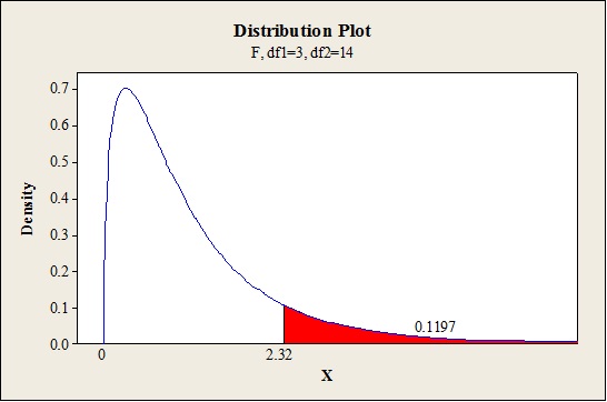
Critical value:
Software procedure:
- Click on Graph, select View Probability and click OK.
- Select F, enter 3 in numerator df and 14 in denominator df.
- Under Shaded Area Tab select Probability under Define Shaded Area By and select Right tail.
- Choose X Value as 2.32.
- Click OK.
Output obtained from MINITAB is given below:
Conclusion:
The P-value is 0.1197 and the level of significance is 0.05.
The P-value is lesser than the level of significance.
That is,
Thus, the null hypothesis is not rejected.
Hence, there is no sufficient evidence to conclude that there is a use of linear relationship betweenspecific gravity and at least one of the predictor percentage of springwood and light absorption in summerwood at 5% level of significance.
Thus, the variables
d.
Predict the value of specific gravity when the percentage of springwood is 50 and percentage of light absorption in summerwood is 90.
d.
Answer to Problem 56E
The estimated value for specific gravity when the percentage of springwood is 50 and percentage of light absorption in summerwood is 90 is 0.5386.
Explanation of Solution
Given info:
The mean and standard deviation for the variable
The estimated regression equation after standardization is
Calculation:
The standardized values
Where,
The standardized value when mean and standard deviation for the variable
Thus, the value of
The standardized value when the mean and standard deviation for the variable
Thus, the value of
The estimated value for specific gravity is,
Thus, the estimated value for specific gravity when the percentage of springwood is 50 and percentage of light absorption in summerwood is 90 is 0.5386.
e.
Find the 95% confidence interval for the estimated coefficient of
e.
Answer to Problem 56E
The 95% confidence interval for the estimated coefficient of
Explanation of Solution
Calculation:
95% confidence interval:
The confidence interval is calculated using the formula:
Where,
n is the total number of observations.
k is the total number of predictors in the model.
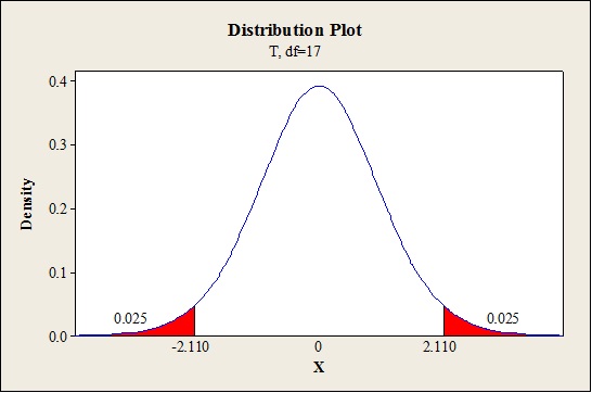
Critical value:
Software procedure:
Step-by-step procedure to find the critical value is given below:
- Click on Graph, select View Probability and click OK.
- Select t, enter 17 as Degrees of freedom, in Shaded Area Tab select Probability under Define Shaded Area By and choose Both tails.
- Enter Probability value as 0.05.
- Click OK.
Output obtained from MINITAB is given below:
The 95% confidence interval is given below:
Thus, the 95% confidence interval for the estimated coefficient of
f.
Find the estimated coefficient and estimated standard deviation of
f.
Answer to Problem 56E
The estimated coefficient of
The estimated standard deviation of
Explanation of Solution
Given info:
Use the information given in part (d) and (e).
Calculation:
The estimated regression equation for standardized model is,
The estimated coefficient of
Thus, the estimated coefficient of
The estimate for
The estimated standard deviation for
Thus, the estimated standard deviation of
g.
Find the 95% prediction interval for the specific gravity when the percentage of spring wood is 50.5 and percentage of light absorption in summerwood is 88.9.
g.
Answer to Problem 56E
The 95% prediction interval for the specific gravity when the percentage of spring wood is 50.5 and percentage of light absorption in summerwood is 88.9 is(0.489, 0.575).
Explanation of Solution
Given info:
The estimated standard deviation for the model with two predictors is 0.02001. The estimated standard deviation for the predicated value when the coefficients
Calculation:
The predicted value for the specific gravity when the percentage of spring wood is 50.5 and percentage of light absorption in summerwood is 88.9 is calculated as follows:
Thus, the predicted value for the specific gravity when the percentage of spring wood is 50.5 and percentage of light absorption in summerwood is 88.9 is 0.532.
95% prediction interval:
The confidence interval is calculated using the formula:
Where,
n is the total number of observations.
k is the total number of predictors in the model.
s is the overall standard deviation obtained after fitting the model.
Critical value:
Software procedure:
Step-by-step procedure to find the critical value is given below:
- Click on Graph, select View Probability and click OK.
- Select t, enter 17 as Degrees of freedom, in Shaded Area Tab select Probability under Define Shaded Area By and choose Both tails.
- Enter Probability value as 0.05.
- Click OK.
Output obtained from MINITAB is given below:
The 95% prediction interval is given below:
Thus, the 95% prediction interval for the specific gravity when the percentage of spring wood is 50.5 and percentage of light absorption in summerwood is 88.9 is (0.489,0.575).
Want to see more full solutions like this?
Chapter 13 Solutions
Bundle: Probability and Statistics for Engineering and the Sciences, 9th + WebAssign Printed Access Card for Devore's Probability and Statistics for ... and the Sciences, 9th Edition, Single-Term


- What would you say about a set of quantitative bivariate data whose linear correlation is -1? What would a scatter diagram of the data look like? (5 points)arrow_forwardBusiness discussarrow_forwardAnalyze the residuals of a linear regression model and select the best response. yes, the residual plot does not show a curve no, the residual plot shows a curve yes, the residual plot shows a curve no, the residual plot does not show a curve I answered, "No, the residual plot shows a curve." (and this was incorrect). I am not sure why I keep getting these wrong when the answer seems obvious. Please help me understand what the yes and no references in the answer.arrow_forward
- a. Find the value of A.b. Find pX(x) and py(y).c. Find pX|y(x|y) and py|X(y|x)d. Are x and y independent? Why or why not?arrow_forwardAnalyze the residuals of a linear regression model and select the best response.Criteria is simple evaluation of possible indications of an exponential model vs. linear model) no, the residual plot does not show a curve yes, the residual plot does not show a curve yes, the residual plot shows a curve no, the residual plot shows a curve I selected: yes, the residual plot shows a curve and it is INCORRECT. Can u help me understand why?arrow_forwardYou have been hired as an intern to run analyses on the data and report the results back to Sarah; the five questions that Sarah needs you to address are given below. please do it step by step on excel Does there appear to be a positive or negative relationship between price and screen size? Use a scatter plot to examine the relationship. Determine and interpret the correlation coefficient between the two variables. In your interpretation, discuss the direction of the relationship (positive, negative, or zero relationship). Also discuss the strength of the relationship. Estimate the relationship between screen size and price using a simple linear regression model and interpret the estimated coefficients. (In your interpretation, tell the dollar amount by which price will change for each unit of increase in screen size). Include the manufacturer dummy variable (Samsung=1, 0 otherwise) and estimate the relationship between screen size, price and manufacturer dummy as a multiple…arrow_forward
- Here is data with as the response variable. x y54.4 19.124.9 99.334.5 9.476.6 0.359.4 4.554.4 0.139.2 56.354 15.773.8 9-156.1 319.2Make a scatter plot of this data. Which point is an outlier? Enter as an ordered pair, e.g., (x,y). (x,y)= Find the regression equation for the data set without the outlier. Enter the equation of the form mx+b rounded to three decimal places. y_wo= Find the regression equation for the data set with the outlier. Enter the equation of the form mx+b rounded to three decimal places. y_w=arrow_forwardYou have been hired as an intern to run analyses on the data and report the results back to Sarah; the five questions that Sarah needs you to address are given below. please do it step by step Does there appear to be a positive or negative relationship between price and screen size? Use a scatter plot to examine the relationship. Determine and interpret the correlation coefficient between the two variables. In your interpretation, discuss the direction of the relationship (positive, negative, or zero relationship). Also discuss the strength of the relationship. Estimate the relationship between screen size and price using a simple linear regression model and interpret the estimated coefficients. (In your interpretation, tell the dollar amount by which price will change for each unit of increase in screen size). Include the manufacturer dummy variable (Samsung=1, 0 otherwise) and estimate the relationship between screen size, price and manufacturer dummy as a multiple linear…arrow_forwardExercises: Find all the whole number solutions of the congruence equation. 1. 3x 8 mod 11 2. 2x+3= 8 mod 12 3. 3x+12= 7 mod 10 4. 4x+6= 5 mod 8 5. 5x+3= 8 mod 12arrow_forward
- Scenario Sales of products by color follow a peculiar, but predictable, pattern that determines how many units will sell in any given year. This pattern is shown below Product Color 1995 1996 1997 Red 28 42 21 1998 23 1999 29 2000 2001 2002 Unit Sales 2003 2004 15 8 4 2 1 2005 2006 discontinued Green 26 39 20 22 28 14 7 4 2 White 43 65 33 36 45 23 12 Brown 58 87 44 48 60 Yellow 37 56 28 31 Black 28 42 21 Orange 19 29 Purple Total 28 42 21 49 68 78 95 123 176 181 164 127 24 179 Questions A) Which color will sell the most units in 2007? B) Which color will sell the most units combined in the 2007 to 2009 period? Please show all your analysis, leave formulas in cells, and specify any assumptions you make.arrow_forwardOne hundred students were surveyed about their preference between dogs and cats. The following two-way table displays data for the sample of students who responded to the survey. Preference Male Female TOTAL Prefers dogs \[36\] \[20\] \[56\] Prefers cats \[10\] \[26\] \[36\] No preference \[2\] \[6\] \[8\] TOTAL \[48\] \[52\] \[100\] problem 1 Find the probability that a randomly selected student prefers dogs.Enter your answer as a fraction or decimal. \[P\left(\text{prefers dogs}\right)=\] Incorrect Check Hide explanation Preference Male Female TOTAL Prefers dogs \[\blueD{36}\] \[\blueD{20}\] \[\blueE{56}\] Prefers cats \[10\] \[26\] \[36\] No preference \[2\] \[6\] \[8\] TOTAL \[48\] \[52\] \[100\] There were \[\blueE{56}\] students in the sample who preferred dogs out of \[100\] total students.arrow_forwardBusiness discussarrow_forward
 MATLAB: An Introduction with ApplicationsStatisticsISBN:9781119256830Author:Amos GilatPublisher:John Wiley & Sons Inc
 Probability and Statistics for Engineering and th...StatisticsISBN:9781305251809Author:Jay L. DevorePublisher:Cengage Learning
 Statistics for The Behavioral Sciences (MindTap C...StatisticsISBN:9781305504912Author:Frederick J Gravetter, Larry B. WallnauPublisher:Cengage Learning
 Elementary Statistics: Picturing the World (7th E...StatisticsISBN:9780134683416Author:Ron Larson, Betsy FarberPublisher:PEARSON
 The Basic Practice of StatisticsStatisticsISBN:9781319042578Author:David S. Moore, William I. Notz, Michael A. FlignerPublisher:W. H. Freeman
 Introduction to the Practice of StatisticsStatisticsISBN:9781319013387Author:David S. Moore, George P. McCabe, Bruce A. CraigPublisher:W. H. Freeman