Concept explainers
Videos
a.
Identify and explain whichof the given modelscan be recommended.
a.
Answer to Problem 66SE
The model with 2 predictors and the model with 3 predictors can be recommended for predicting the pH before addition of dyes.
Explanation of Solution
Given info:
The MINITAB output shows the best regression option for the data predicted for pH before the addition of dyes using carpet density, carpet weight, dye weight, dye weight as a percentage of carpet and pH after addition of dyes.
Justification:
Mallows
It is used to assess the fit of regression model where the aim to find the best subset of predictors. A relatively small value of
By observing the mallows
By examining the models with three variables,
Hence, the model with two predictorsnamely dye weight and pH after addition of dyes could be considered as a best model subset for predicting pH before the addition of dyes.
Also, a second option would be the model with three predictorsnamely carpet weight, dye weight and pH after addition of dyes could be considered as a best model subset for predicting pH before the addition of dyes.
b.
Test whether the model suggests a useful linear relationship between pH before the addition of dyes and at least one of the predictors.
b.
Answer to Problem 66SE
There is sufficient evidence to conclude that the there is a use of linear relationship between pH before the addition of dyes and at least one of the predictors dye weight and pH after the addition of dyes.
Explanation of Solution
Given info:
The MINITAB output for predicting the pH before the addition of dyes using the dye weight
Calculation:
The test hypotheses are given below:
Null hypothesis:
That is, there is no use of linear relationship between pH before the addition of dyes and the predictors dye weightand pH after the addition of dyes.
Alternative hypothesis:
That is, there is a use of linear relationship between pH before the addition of dyes and at least one of the predictors dye weightand pH after the addition of dyes.
Conclusion:
The P-value is 0.000 and the level of significance is 0.001.
The P-value is lesser than the level of significance.
That is
Thus, the null hypothesis is rejected.
Hence, there is sufficient evidence to conclude that there is a use of linear relationship between pH before the addition of dyes and at least one of the predictors dye weight and pH after the addition of dyes.
c.
Explain whether either one of the predictors could be eliminated from the model given that the other predictor is retained.
c.
Answer to Problem 66SE
No, either one of the predictors could not be eliminated from the model given that the other predictor is retained.
Explanation of Solution
Calculation:
For variable
Testing the hypothesis:
Null hypothesis:
That is, there is no use of linear relationship between pH before the addition of dyes and dye weightgiven that pH after addition of dyes was retained in the model.
Alternative hypothesis:
That is, there is a use of linear relationship between pH before the addition of dyes and dye weightgiven that pH after addition of dyes was retained in the model.
From the MINITAB output it can be observed that the P-value corresponding to the t statistic of
Conclusion:
The P-value is 0.000 and the level of significance is 0.001.
The P-value is lesser than the level of significance.
That is
Thus, the null hypothesis is rejected.
Hence, there is sufficient evidence to conclude that there is a use of linear relationship between pH before the addition of dyes and dye weight given that pH after addition of dyes was retained in the model.
For variable
Testing the hypothesis:
Null hypothesis:
That is, there is no use of linear relationship between pH before the addition of dyes and pH after addition of dyes given that dye weight was retained in the model.
Alternative hypothesis:
That is, there is a use of linear relationship between pH before the addition of dyes and pH after addition of dyes given that dye weight was retained in the model.
From the MINITAB output it can be observed that the P-value corresponding to the t statistic of
Conclusion:
The P-value is 0.000 and the level of significance is 0.001.
The P-value is lesser than the level of significance.
That is
Thus, the null hypothesis is rejected.
Hence, there is sufficient evidence to conclude that there is a use of linear relationship between pH before the addition of dyes and pH after addition of dyes given that dye weight was retained in the model.
Justification:
From the analysis it can be concluded that none of the variables can be eliminated from the model given that the other variable is already present in the model.
d.
Calculate and interpret the 95% confidence interval for the two predictors.
d.
Answer to Problem 66SE
The 95% confidence interval for the estimated slope coefficient
(–0.0000684, –0.0000244).
The 95% confidence interval for the estimated slope coefficient
Explanation of Solution
Calculation:
The 95% confidence interval is calculated using the formula:
The confidence interval is calculated using the formula:
Where,
n is the total number of observations.
k is the total number of predictors in the model.
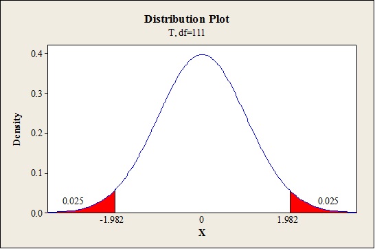
Critical value:
Software procedure:
Step-by-step procedure to find the critical value is given below:
- Click on Graph, select View Probability and click OK.
- Select t, enter 111 as Degrees of freedom, inShaded Area Tab select Probability under Define Shaded Area By and choose Both tails.
- Enter Probability value as 0.05.
- Click OK.
Output obtained from MINITAB is given below:
The 95% confidence interval for
Thus, the 95% confidence interval for the estimated slope coefficient
(–0.0000684, –0.0000244).
The 95% confidence interval for
Thus, the 95% confidence interval for the estimated slope coefficient
(0.6417,0.8325).
Interpretation:
For the variable
For one unit increase in the dye weight, it is 95% confident that the estimated value of pH before addition of dyes would decrease between–0.00000684 and–0.0000244 given that pH after addition of dyes is fixed constant.
For the variable
For one unit increase in the pH after the addition of dyes it is 95% confident that the estimated value of pH before addition of dyes would increase between 0.6417 and 0.8325 given that dye weight is fixed constant.
e.
Calculate and interpret the 95% confidence interval for the average value of pH before the addition of dyes when the dye weight and pH after the addition of dyes takes 1,000 and 6, respectively.
e.
Answer to Problem 66SE
The 95% confidence interval for the average value of pH before the addition of dyes when the dye weight and pH after the addition of dyes takes 1,000 and 6, respectively is (5.250, 5.383)
Explanation of Solution
Given info:
The estimated standard deviation for predicting the pH before the addition of dyes when the dye weight and pH after the addition of dyes takes 1,000 and 6 is 0.0336.
Calculation:
The average value of pH before the addition of dyes when the dye weight and pH after the addition of dyes takes 1,000 and 6 is calculated as follows:
Thus, the average value of pH before the addition of dyes when the dye weight and pH after the addition of dyes takes 1,000 and 6 is 5.316.
95% confidence interval for the true response:
The confidence interval is calculated using the formula:
Where,
n is the total number of observations.
k is the total number of predictors in the model.
Critical value:
Software procedure:
Step-by-step procedure to find the critical value is given below:
- Click on Graph, select View Probability and click OK.
- Select t, enter 111 as Degrees of freedom, in Shaded Area Tab select Probability under Define Shaded Area By and choose Both tails.
- Enter Probability value as 0.05.
- Click OK.
Output obtained from MINITAB is given below:
The 95% confidence interval is given below:
Thus, the 95% confidence interval for the average value of pH before the addition of dyes when the dye weight and pH after the addition of dyes takes 1,000 and 6 is (5.250,5.383).
Interpretation:
It is 95% confident that average value of pH before the addition of dyes when the dye weight and pH after the addition of dyes takes 1,000 and 6 would lie between 5.250 and 5.383.
Want to see more full solutions like this?
Chapter 13 Solutions
EBK PROBABILITY AND STATISTICS FOR ENGI


- The table below was compiled for a middle school from the 2003 English/Language Arts PACT exam. Grade 6 7 8 Below Basic 60 62 76 Basic 87 134 140 Proficient 87 102 100 Advanced 42 24 21 Partition the likelihood ratio test statistic into 6 independent 1 df components. What conclusions can you draw from these components?arrow_forwardWhat is the value of the maximum likelihood estimate, θ, of θ based on these data? Justify your answer. What does the value of θ suggest about the value of θ for this biased die compared with the value of θ associated with a fair, unbiased, die?arrow_forwardShow that L′(θ) = Cθ394(1 −2θ)604(395 −2000θ).arrow_forward
- a) Let X and Y be independent random variables both with the same mean µ=0. Define a new random variable W = aX +bY, where a and b are constants. (i) Obtain an expression for E(W).arrow_forwardThe table below shows the estimated effects for a logistic regression model with squamous cell esophageal cancer (Y = 1, yes; Y = 0, no) as the response. Smoking status (S) equals 1 for at least one pack per day and 0 otherwise, alcohol consumption (A) equals the average number of alcohoic drinks consumed per day, and race (R) equals 1 for blacks and 0 for whites. Variable Effect (β) P-value Intercept -7.00 <0.01 Alcohol use 0.10 0.03 Smoking 1.20 <0.01 Race 0.30 0.02 Race × smoking 0.20 0.04 Write-out the prediction equation (i.e., the logistic regression model) when R = 0 and again when R = 1. Find the fitted Y S conditional odds ratio in each case. Next, write-out the logistic regression model when S = 0 and again when S = 1. Find the fitted Y R conditional odds ratio in each case.arrow_forwardThe chi-squared goodness-of-fit test can be used to test if data comes from a specific continuous distribution by binning the data to make it categorical. Using the OpenIntro Statistics county_complete dataset, test the hypothesis that the persons_per_household 2019 values come from a normal distribution with mean and standard deviation equal to that variable's mean and standard deviation. Use signficance level a = 0.01. In your solution you should 1. Formulate the hypotheses 2. Fill in this table Range (-⁰⁰, 2.34] (2.34, 2.81] (2.81, 3.27] (3.27,00) Observed 802 Expected 854.2 The first row has been filled in. That should give you a hint for how to calculate the expected frequencies. Remember that the expected frequencies are calculated under the assumption that the null hypothesis is true. FYI, the bounderies for each range were obtained using JASP's drag-and-drop cut function with 8 levels. Then some of the groups were merged. 3. Check any conditions required by the chi-squared…arrow_forward
- Suppose that you want to estimate the mean monthly gross income of all households in your local community. You decide to estimate this population parameter by calling 150 randomly selected residents and asking each individual to report the household’s monthly income. Assume that you use the local phone directory as the frame in selecting the households to be included in your sample. What are some possible sources of error that might arise in your effort to estimate the population mean?arrow_forwardFor the distribution shown, match the letter to the measure of central tendency. A B C C Drag each of the letters into the appropriate measure of central tendency. Mean C Median A Mode Barrow_forwardA physician who has a group of 38 female patients aged 18 to 24 on a special diet wishes to estimate the effect of the diet on total serum cholesterol. For this group, their average serum cholesterol is 188.4 (measured in mg/100mL). Suppose that the total serum cholesterol measurements are normally distributed with standard deviation of 40.7. (a) Find a 95% confidence interval of the mean serum cholesterol of patients on the special diet.arrow_forward
- The accompanying data represent the weights (in grams) of a simple random sample of 10 M&M plain candies. Determine the shape of the distribution of weights of M&Ms by drawing a frequency histogram. Find the mean and median. Which measure of central tendency better describes the weight of a plain M&M? Click the icon to view the candy weight data. Draw a frequency histogram. Choose the correct graph below. ○ A. ○ C. Frequency Weight of Plain M and Ms 0.78 0.84 Frequency OONAG 0.78 B. 0.9 0.96 Weight (grams) Weight of Plain M and Ms 0.84 0.9 0.96 Weight (grams) ○ D. Candy Weights 0.85 0.79 0.85 0.89 0.94 0.86 0.91 0.86 0.87 0.87 - Frequency ☑ Frequency 67200 0.78 → Weight of Plain M and Ms 0.9 0.96 0.84 Weight (grams) Weight of Plain M and Ms 0.78 0.84 Weight (grams) 0.9 0.96 →arrow_forwardThe acidity or alkalinity of a solution is measured using pH. A pH less than 7 is acidic; a pH greater than 7 is alkaline. The accompanying data represent the pH in samples of bottled water and tap water. Complete parts (a) and (b). Click the icon to view the data table. (a) Determine the mean, median, and mode pH for each type of water. Comment on the differences between the two water types. Select the correct choice below and fill in any answer boxes in your choice. A. For tap water, the mean pH is (Round to three decimal places as needed.) B. The mean does not exist. Data table Тар 7.64 7.45 7.45 7.10 7.46 7.50 7.68 7.69 7.56 7.46 7.52 7.46 5.15 5.09 5.31 5.20 4.78 5.23 Bottled 5.52 5.31 5.13 5.31 5.21 5.24 - ☑arrow_forwardく Chapter 5-Section 1 Homework X MindTap - Cengage Learning x + C webassign.net/web/Student/Assignment-Responses/submit?pos=3&dep=36701632&tags=autosave #question3874894_3 M Gmail 品 YouTube Maps 5. [-/20 Points] DETAILS MY NOTES BBUNDERSTAT12 5.1.020. ☆ B Verify it's you Finish update: All Bookmarks PRACTICE ANOTHER A computer repair shop has two work centers. The first center examines the computer to see what is wrong, and the second center repairs the computer. Let x₁ and x2 be random variables representing the lengths of time in minutes to examine a computer (✗₁) and to repair a computer (x2). Assume x and x, are independent random variables. Long-term history has shown the following times. 01 Examine computer, x₁₁ = 29.6 minutes; σ₁ = 8.1 minutes Repair computer, X2: μ₂ = 92.5 minutes; σ2 = 14.5 minutes (a) Let W = x₁ + x2 be a random variable representing the total time to examine and repair the computer. Compute the mean, variance, and standard deviation of W. (Round your answers…arrow_forward
 Big Ideas Math A Bridge To Success Algebra 1: Stu...AlgebraISBN:9781680331141Author:HOUGHTON MIFFLIN HARCOURTPublisher:Houghton Mifflin Harcourt