Concept explainers
Videos
(a)
To find: The means for each species by water combination and plot these means.
(a)
Answer to Problem 51E
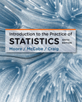
Solution: For Fresh biomass, the first three means for Species-1 are 109.1, 165.1, and 168.82. The first three means for Species-2 are 116.4, 156.8, and 254.88. The first three means for Species-3 are 55.60, 78.9, and 90.3. The first three means for Species-4 are 35.13, 58.33, and 94.54.
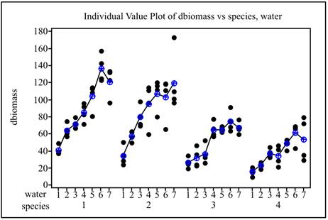
For Dry biomass, the first three means for Species-1 are 40.56, 63.86, and 71.00. The first three means for Species-2 are 34.50, 57.36, and 79.60. The first three means for Species-3 are 26.25, 31.87, and 36.24. The first three means for Species-4 are 15.53, 23.29, and 37.05.
Explanation of Solution
Calculation: To obtain the means for the response variable Fresh biomass, Minitab is used. The steps to be followed are:
Step 1: Go to the Minitab worksheet.
Step 2: Go to Stat
Step 3: Enter the variable ‘Fresh biomass’ in the ‘Variable’ option.
Step 4: Enter the variables ‘Species and Water’ in the ‘By Variable’ option.
Step 5: Go to statistics and select ‘Mean.
Step 6: Go to graph and select Individual value plot’.
Step 7: Click Ok.
The obtained result shows the means for each species by water level. Here, few of them are given: The first three means for Species-1 are 109.1, 165.1, and 168.82. The first three means for Species-2 are 116.4, 156.8, and 254.88. The first three means for species-3 are 55.60, 78.9, and 90.3. The first three means for Species-4 are 35.13, 58.33, and 94.54. The obtained graph is given below:
To obtain the means for the response variable Dry biomass, Minitab is used. The steps to be followed are:
Step 1: Go to the Minitab worksheet.
Step 2: Go to Stat
Step 3: Enter the variable ‘Dry biomass’ in the ‘Variable’ option.
Step 4: Enter the variables ‘Species and Water’ in the ‘By Variable’ option.
Step 5: Go to statistics and select ‘Mean.
Step 6: Go to graph and select Individual value plot’.
Step 7: Click Ok.
The obtained result shows the means for each species by water level. Here, few of them are given: The first three means for Species-1 are 40.56, 63.86, and 71.00. The first three means for Species-2 are 34.50, 57.36, and 79.60. The first three means for species-3 are 26.25, 31.87, and 36.24. The first three means for Species-4 are 15.53, 23.29, and 37.05. The obtained graph is given below:
(b)
To find: The standard deviation for each species by water combination and plot these means.
(b)
Answer to Problem 51E
Solution: For Fresh biomass, the first three standard deviations for Species-1 are 20.9, 29.1, and 18.87. The first three standard deviations for Species-2 are 29.3, 46.9, and 13.94. The first three standard deviations for Species-3 are 13.20, 29.5, and 28.3. The first three standard deviations for Species-4 are 11.63, 6.79, and 13.93.
For Dry biomass, the first three standard deviations for Species-1 are 5.58, 7.51, and 6.03. The first three standard deviations for Species-2 are 11.61, 6.15, and 13.09. The first three standard deviations for Species-3 are 6.43, 11.32, and 11.27. The first three standard deviations for Species-4 are 4.89, 3.33, and 5.19.
Explanation of Solution
Calculation: To obtain the means for Fresh biomass, Minitab is used. The steps to be followed are:
Step 1: Go to the Minitab worksheet.
Step 2: Go to Stat
Step 3: Enter the variable ‘Fresh biomass’ in the ‘Variable’ option.
Step 4: Enter the variables ‘Species and Water’ in the ‘By Variable’ option.
Step 5: Go to statistics and select ‘Standard deviation’.
Step 6: Click Ok.
The obtained result shows the means for each species by water level. Here, few of them are given: The first three standard deviations for Species-1 are 20.9, 29.1, and 18.87. The first three standard deviations for Species-2 are 29.3, 46.9, and 13.94. The first three standard deviations for species-3 are 13.20, 29.5, and 28.3. The first three standard deviations for Species-4 are 11.63, 6.79, and 13.93.
To obtain the means for Dry biomass, Minitab is used. The steps to be followed are:
Step 1: Go to the Minitab worksheet.
Step 2: Go to Stat
Step 3: Enter the variable ‘Dry biomass’ in the ‘Variable’ option.
Step 4: Enter the variables ‘Species and Water’ in the ‘By Variable’ option.
Step 5: Go to statistics and select ‘Standard deviation’.
Step 6: Click Ok.
The obtained result shows the means for each species by water level. Here, few of them are given: The first three standard deviations for Species-1 are 5.58, 7.51, and 6.03. The first three standard deviations for Species-2 are 11.61, 6.15, and 13.09. The first three standard deviations for species-3 are 6.43, 11.32, and 11.27. The first three standard deviations for Species-4 are 4.89, 3.33, and 5.19
The highest SD from the Fresh biomass data is 108.01 and the lowest SD is 6.79. Thus,
The highest SD from the Dry biomass data is 35.76 and the lowest SD is 3.12. Thus,
Hence, it is reasonable to pool the standard deviation.
(c)
To test: A two-way ANOVA for Fresh biomass and Dry biomass
(c)
Answer to Problem 51E
Solution: A two-way ANOVA for Fresh biomass is provided below:
Source of Variation |
Degree of freedom |
Sum of squares |
Mean sum of squares |
F- value |
P- value |
Species |
3 |
458295 |
152765 |
81.45 |
0.000 |
Water |
6 |
491948 |
81991 |
43.71 |
0.000 |
Interaction |
18 |
60334 |
3352 |
1.79 |
0.040 |
Error |
84 |
157551 |
1876 |
||
Total |
111 |
1168129 |
A two-way ANOVA for Dry biomass is provided below:
Source of Variation |
Degree of freedom |
Sum of squares |
Mean sum of squares |
F- value |
P- value |
Species |
3 |
50524 |
16841.3 |
79.93 |
0.000 |
Water |
6 |
56624 |
9437.3 |
44.79 |
0.000 |
Interaction |
18 |
8419 |
467.7 |
2.22 |
0.008 |
Error |
84 |
17698 |
219.7 |
||
Total |
111 |
133265 |
Explanation of Solution
Calculation: To perform a Two-way ANOVA for Fresh biomass, Minitab is used. The steps to be followed are:
Step 1: Go to the Minitab worksheet.
Step 2: Go to Stat
Step 3: Enter the variable ‘Fresh biomass’ in the ‘Response’ option.
Step 4: Enter the variables ‘Species’ in the ‘Row Factor and ‘Water’ in the Column Factor’.
Step 5: Click Ok.
The obtained results are provided below:
Source of Variation |
Degree of freedom |
Sum of squares |
Mean sum of squares |
F- value |
P- value |
Species |
3 |
458295 |
152765 |
81.45 |
0.000 |
Water |
6 |
491948 |
81991 |
43.71 |
0.000 |
Interaction |
18 |
60334 |
3352 |
1.79 |
0.040 |
Error |
84 |
157551 |
1876 |
||
Total |
111 |
1168129 |
To perform a Two-way ANOVA for Dry biomass, Minitab is used. The steps to be followed are:
Step 1: Go to the Minitab worksheet.
Step 2: Go to Stat
Step 3: Enter the variable ‘Dry biomass’ in the ‘Response’ option.
Step 4: Enter the variables ‘Species’ in the ‘Row Factor and ‘Water’ in the Column Factor’.
Step 5: Click Ok.
The obtained results are provided below:
Source of Variation |
Degree of freedom |
Sum of squares |
Mean sum of squares |
F- value |
P- value |
Species |
3 |
50524 |
16841.3 |
79.93 |
0.000 |
Water |
6 |
56624 |
9437.3 |
44.79 |
0.000 |
Interaction |
18 |
8419 |
467.7 |
2.22 |
0.008 |
Error |
84 |
17698 |
219.7 |
||
Total |
111 |
133265 |
Conclusion: From ANOVA table above, for both Fresh biomass and Dry biomass, main effects and interaction are significant. The interaction for Fresh biomass and Dry biomass has the P-value 0.04 and 0.008, respectively.
Want to see more full solutions like this?
Chapter 13 Solutions
Introduction to the Practice of Statistics


- For each of the time series, construct a line chart of the data and identify the characteristics of the time series (that is, random, stationary, trend, seasonal, or cyclical). Year Month Units1 Nov 42,1611 Dec 44,1862 Jan 42,2272 Feb 45,4222 Mar 54,0752 Apr 50,9262 May 53,5722 Jun 54,9202 Jul 54,4492 Aug 56,0792 Sep 52,1772 Oct 50,0872 Nov 48,5132 Dec 49,2783 Jan 48,1343 Feb 54,8873 Mar 61,0643 Apr 53,3503 May 59,4673 Jun 59,3703 Jul 55,0883 Aug 59,3493 Sep 54,4723 Oct 53,164arrow_forwardHigh Cholesterol: A group of eight individuals with high cholesterol levels were given a new drug that was designed to lower cholesterol levels. Cholesterol levels, in milligrams per deciliter, were measured before and after treatment for each individual, with the following results: Individual Before 1 2 3 4 5 6 7 8 237 282 278 297 243 228 298 269 After 200 208 178 212 174 201 189 185 Part: 0/2 Part 1 of 2 (a) Construct a 99.9% confidence interval for the mean reduction in cholesterol level. Let a represent the cholesterol level before treatment minus the cholesterol level after. Use tables to find the critical value and round the answers to at least one decimal place.arrow_forwardI worked out the answers for most of this, and provided the answers in the tables that follow. But for the total cost table, I need help working out the values for 10%, 11%, and 12%. A pharmaceutical company produces the drug NasaMist from four chemicals. Today, the company must produce 1000 pounds of the drug. The three active ingredients in NasaMist are A, B, and C. By weight, at least 8% of NasaMist must consist of A, at least 4% of B, and at least 2% of C. The cost per pound of each chemical and the amount of each active ingredient in one pound of each chemical are given in the data at the bottom. It is necessary that at least 100 pounds of chemical 2 and at least 450 pounds of chemical 3 be used. a. Determine the cheapest way of producing today’s batch of NasaMist. If needed, round your answers to one decimal digit. Production plan Weight (lbs) Chemical 1 257.1 Chemical 2 100 Chemical 3 450 Chemical 4 192.9 b. Use SolverTable to see how much the percentage of…arrow_forward
- At the beginning of year 1, you have $10,000. Investments A and B are available; their cash flows per dollars invested are shown in the table below. Assume that any money not invested in A or B earns interest at an annual rate of 2%. a. What is the maximized amount of cash on hand at the beginning of year 4.$ ___________ A B Time 0 -$1.00 $0.00 Time 1 $0.20 -$1.00 Time 2 $1.50 $0.00 Time 3 $0.00 $1.90arrow_forwardFor each of the time series, construct a line chart of the data and identify the characteristics of the time series (that is, random, stationary, trend, seasonal, or cyclical). Year Month Rate (%)2009 Mar 8.72009 Apr 9.02009 May 9.42009 Jun 9.52009 Jul 9.52009 Aug 9.62009 Sep 9.82009 Oct 10.02009 Nov 9.92009 Dec 9.92010 Jan 9.82010 Feb 9.82010 Mar 9.92010 Apr 9.92010 May 9.62010 Jun 9.42010 Jul 9.52010 Aug 9.52010 Sep 9.52010 Oct 9.52010 Nov 9.82010 Dec 9.32011 Jan 9.12011 Feb 9.02011 Mar 8.92011 Apr 9.02011 May 9.02011 Jun 9.12011 Jul 9.02011 Aug 9.02011 Sep 9.02011 Oct 8.92011 Nov 8.62011 Dec 8.52012 Jan 8.32012 Feb 8.32012 Mar 8.22012 Apr 8.12012 May 8.22012 Jun 8.22012 Jul 8.22012 Aug 8.12012 Sep 7.82012 Oct…arrow_forwardFor each of the time series, construct a line chart of the data and identify the characteristics of the time series (that is, random, stationary, trend, seasonal, or cyclical). Date IBM9/7/2010 $125.959/8/2010 $126.089/9/2010 $126.369/10/2010 $127.999/13/2010 $129.619/14/2010 $128.859/15/2010 $129.439/16/2010 $129.679/17/2010 $130.199/20/2010 $131.79 a. Construct a line chart of the closing stock prices data. Choose the correct chart below.arrow_forward
- For each of the time series, construct a line chart of the data and identify the characteristics of the time series (that is, random, stationary, trend, seasonal, or cyclical) Date IBM9/7/2010 $125.959/8/2010 $126.089/9/2010 $126.369/10/2010 $127.999/13/2010 $129.619/14/2010 $128.859/15/2010 $129.439/16/2010 $129.679/17/2010 $130.199/20/2010 $131.79arrow_forward1. A consumer group claims that the mean annual consumption of cheddar cheese by a person in the United States is at most 10.3 pounds. A random sample of 100 people in the United States has a mean annual cheddar cheese consumption of 9.9 pounds. Assume the population standard deviation is 2.1 pounds. At a = 0.05, can you reject the claim? (Adapted from U.S. Department of Agriculture) State the hypotheses: Calculate the test statistic: Calculate the P-value: Conclusion (reject or fail to reject Ho): 2. The CEO of a manufacturing facility claims that the mean workday of the company's assembly line employees is less than 8.5 hours. A random sample of 25 of the company's assembly line employees has a mean workday of 8.2 hours. Assume the population standard deviation is 0.5 hour and the population is normally distributed. At a = 0.01, test the CEO's claim. State the hypotheses: Calculate the test statistic: Calculate the P-value: Conclusion (reject or fail to reject Ho): Statisticsarrow_forward21. find the mean. and variance of the following: Ⓒ x(t) = Ut +V, and V indepriv. s.t U.VN NL0, 63). X(t) = t² + Ut +V, U and V incepires have N (0,8) Ut ①xt = e UNN (0162) ~ X+ = UCOSTE, UNNL0, 62) SU, Oct ⑤Xt= 7 where U. Vindp.rus +> ½ have NL, 62). ⑥Xn = ΣY, 41, 42, 43, ... Yn vandom sample K=1 Text with mean zen and variance 6arrow_forward
- A psychology researcher conducted a Chi-Square Test of Independence to examine whether there is a relationship between college students’ year in school (Freshman, Sophomore, Junior, Senior) and their preferred coping strategy for academic stress (Problem-Focused, Emotion-Focused, Avoidance). The test yielded the following result: image.png Interpret the results of this analysis. In your response, clearly explain: Whether the result is statistically significant and why. What this means about the relationship between year in school and coping strategy. What the researcher should conclude based on these findings.arrow_forwardA school counselor is conducting a research study to examine whether there is a relationship between the number of times teenagers report vaping per week and their academic performance, measured by GPA. The counselor collects data from a sample of high school students. Write the null and alternative hypotheses for this study. Clearly state your hypotheses in terms of the correlation between vaping frequency and academic performance. EditViewInsertFormatToolsTable 12pt Paragrapharrow_forwardA smallish urn contains 25 small plastic bunnies – 7 of which are pink and 18 of which are white. 10 bunnies are drawn from the urn at random with replacement, and X is the number of pink bunnies that are drawn. (a) P(X = 5) ≈ (b) P(X<6) ≈ The Whoville small urn contains 100 marbles – 60 blue and 40 orange. The Grinch sneaks in one night and grabs a simple random sample (without replacement) of 15 marbles. (a) The probability that the Grinch gets exactly 6 blue marbles is [ Select ] ["≈ 0.054", "≈ 0.043", "≈ 0.061"] . (b) The probability that the Grinch gets at least 7 blue marbles is [ Select ] ["≈ 0.922", "≈ 0.905", "≈ 0.893"] . (c) The probability that the Grinch gets between 8 and 12 blue marbles (inclusive) is [ Select ] ["≈ 0.801", "≈ 0.760", "≈ 0.786"] . The Whoville small urn contains 100 marbles – 60 blue and 40 orange. The Grinch sneaks in one night and grabs a simple random sample (without replacement) of 15 marbles. (a)…arrow_forward
 MATLAB: An Introduction with ApplicationsStatisticsISBN:9781119256830Author:Amos GilatPublisher:John Wiley & Sons Inc
 Probability and Statistics for Engineering and th...StatisticsISBN:9781305251809Author:Jay L. DevorePublisher:Cengage Learning
 Statistics for The Behavioral Sciences (MindTap C...StatisticsISBN:9781305504912Author:Frederick J Gravetter, Larry B. WallnauPublisher:Cengage Learning
 Elementary Statistics: Picturing the World (7th E...StatisticsISBN:9780134683416Author:Ron Larson, Betsy FarberPublisher:PEARSON
 The Basic Practice of StatisticsStatisticsISBN:9781319042578Author:David S. Moore, William I. Notz, Michael A. FlignerPublisher:W. H. Freeman
 Introduction to the Practice of StatisticsStatisticsISBN:9781319013387Author:David S. Moore, George P. McCabe, Bruce A. CraigPublisher:W. H. Freeman