
Sub part (a):
Consumption schedule and marginal propensity to consume.
Sub part (a):
Explanation of Solution
Table -1 shows the consumption schedule:
Table -1
|
| Consumption |
| 100 | 120 |
| 200 | 200 |
| 300 | 280 |
| 400 | 360 |
| 500 | 440 |
| 600 | 520 |
| 700 | 600 |
Figure 1 illustrates the level of consumption at different level of gross domestic product (GDP).
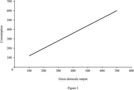
In Figure 1, the horizontal axis measures the gross domestic output and the vertical axis measures the consumption level.
Size of marginal propensity to consume (MPC) can be calculated as follows.
The size of marginal propensity to consume is 0.8.
Concept introduction:
Consumption schedule: Consumption schedule refers to the quantity of consumption at different levels of income.
Marginal propensity to consume (MPS): Marginal propensity to consume refers to the sensitivity of change in the consumption level due to the changes occurred in the income level.
Sub part (b):
Disposable income, tax rate, consumption schedule, marginal propensity to consume and multiplier.
Sub part (b):
Explanation of Solution
Disposable income (DI) can be calculated by using the following formula.
Substitute the respective values in Equation (1) to calculate the disposable income at the level of GDP $100.
Disposable income at the level of GDP $100 is $90.
Tax rate can be calculated by using the following formula.
Substitute the respective values in Equation (2) to calculate the tax rate at the level of GDP $100.
Tax rate at the level of GDP is 10%.
New consumption level can be calculated by using the following formula.
Substitute the respective values in Equation (3) to calculate the disposable income at the level of GDP $100. Since, the tax payment is equal amount of decrease in consumption for all the levels of GDP. The decreasing consumption for increasing $10 is assumed to be $8.
New consumption is $112.
Table -2 shows the values of disposable income, new consumption level after tax and the tax rate that are obtained by using Equations (1), (2) and (3).
Table -2
| Gross domestic product | Tax | DI | New consumption | Tax rate |
| 100 | 10 | 90 | 112 | 10% |
| 200 | 10 | 190 | 192 | 5% |
| 300 | 10 | 290 | 272 | 3.33% |
| 400 | 10 | 390 | 352 | 2.5% |
| 500 | 10 | 490 | 432 | 2% |
| 600 | 10 | 590 | 512 | 1.67% |
| 700 | 10 | 690 | 592 | 1.43% |
Size of marginal propensity to consume (MPC) can be calculated as follows.
The size of marginal propensity to consume is 0.8.
Multiplier: Multiplier refers to the ratio of change in the real GDP to the change in initial consumption, at a constant price rate. Multiplier is positively related to the marginal propensity to consumer and negatively related with the marginal propensity to save. Multiplier can be evaluated using the following formula:
Since the value of MPC remains the same for part (a) and part (b), there is no change in the value of multiplier. The value of multiplier is 5
Figure -2 illustrates the level of consumption at different level of gross domestic product (GDP) for lump sum tax (Regressive tax).
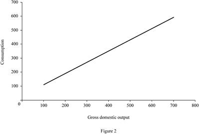
In Figure -2, the horizontal axis measures the gross domestic output and the vertical axis measures the consumption level.
Concept introduction:
Consumption schedule: Consumption schedule refers to the quantity of consumption at different levels of income.
Marginal propensity to consume (MPS): Marginal propensity to consume refers to the sensitivity of change in the consumption level due to the changes occurred in the income level.
Multiplier: Multiplier refers to the ratio of change in the real GDP to the change in initial consumption at constant price rate. Multiplier is positively related to the marginal propensity to consumer and negatively related with the marginal propensity to save.
Sub part (c):
Tax amount, consumption schedule, marginal propensity to consume and multiplier.
Sub part (c):
Explanation of Solution
Tax amount can be calculated by using the following formula.
Substitute the respective values in Equation (4) to calculate the tax amount at $100 GDP.
Tax amount is $10.
Table -3 shows the values of disposable income, new consumption level after tax and the tax rate that are obtained by using Equations (1), (2), (3) and (4). The change in tax amount is differing for different levels of GDP. The decreasing consumption for increasing each $10 is assumed to be $8 (Thus, if the tax payment is $30, then the consumption decreases by $24
Table -3
| Gross domestic product | Tax | DI | New consumption | Tax rate |
| 100 | 10 | 90 | 112 | 10% |
| 200 | 20 | 180 | 184 | 10% |
| 300 | 30 | 270 | 256 | 10% |
| 400 | 40 | 360 | 328 | 10% |
| 500 | 50 | 450 | 400 | 10% |
| 600 | 60 | 540 | 472 | 10% |
| 700 | 70 | 630 | 544 | 10% |
Multiplier: Multiplier refers to the ratio of change in the real GDP to the change in initial consumption, at a constant price rate. Multiplier is positively related to the marginal propensity to consumer and negatively related with the marginal propensity to save. Multiplier can be evaluated using the following formula:
Since the value of MPC different for part (a) and part (c), the value of multiplier for both the part is different. The value of multiplier is 3.57
Figure -3 illustrates the level of consumption at different level of gross domestic product (GDP) for proportional tax.
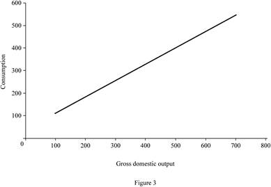
In Figure -3, the horizontal axis measures the gross domestic output and the vertical axis measures the consumption level.
Concept introduction:
Consumption schedule: Consumption schedule refers to the quantity of consumption at different levels of income.
Marginal propensity to consume (MPS): Marginal propensity to consume refers to the sensitivity of change in the consumption level due to the changes occurred in the income level.
Multiplier: Multiplier refers to the ratio of change in the real GDP to the change in initial consumption at constant price rate. Multiplier is positively related to the marginal propensity to consumer and negatively related with the marginal propensity to save.
Sub part (d):
consumption schedule, marginal propensity to consume and multiplier.
Sub part (d):
Explanation of Solution
Marginal propensity to consume can be calculated by using the following formula.
Substitute the respective values in Equation (5) to calculate the MPC at $100 GDP.
The value of MPC is 0.72.
Table -4 shows the values of disposable income, new consumption level after tax and the tax rate that are obtained by using Equations (1), (2), (3), (4) and (5). The change in tax amount is differing for different levels of GDP. The decreasing consumption for increasing each $10 is assumed to be $8 (Thus, if the tax payment is $20, then the consumption decreases by $16
Table -3
| Gross domestic product | Tax | DI | New consumption | Tax rate | MPC |
| 100 | 0 | 100 | 120 | 0% | |
| 200 | 10 | 190 | 192 | 5% | 0.8 |
| 300 | 30 | 270 | 256 | 10% | 0.64 |
| 400 | 60 | 340 | 312 | 15% | 0.56 |
| 500 | 100 | 400 | 360 | 20% | 0.48 |
| 600 | 150 | 450 | 400 | 25% | 0.4 |
| 700 | 210 | 490 | 432 | 30% | 0.32 |
Multiplier: Multiplier refers to the ratio of change in the real GDP to the change in initial consumption, at a constant price rate. Multiplier is positively related to the marginal propensity to consumer and negatively related with the marginal propensity to save.
Multiplier value is differing for each level of GDP. When the tax rate increases, it reduces the value of MPC. Since the value of MPC decreases, the value of multiplier will also decrease.
Figure 4 illustrates the level of consumption at different level of gross domestic product (GDP) for progressive tax.
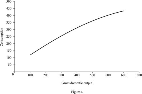
In Figure 4, the horizontal axis measures the gross domestic output and the vertical axis measures the consumption level.
Concept introduction:
Consumption schedule: Consumption schedule refers to the quantity of consumption at different levels of income.
Marginal propensity to consume (MPS): Marginal propensity to consume refers to the sensitivity of change in the consumption level due to the changes occurred in the income level.
Multiplier: Multiplier refers to the ratio of change in the real GDP to the change in initial consumption at constant price rate. Multiplier is positively related to the marginal propensity to consumer and negatively related with the marginal propensity to save.
Sup part (e):
Marginal propensity to consume and multiplier.
Sup part (e):
Explanation of Solution
Figure 1, Figure 2, Figure 3 and Figure 4 reveals that the proportional and progressive tax system reduces the value of MPC, so that the value of multiplier also decreases. The regressive tax system (Lump sum tax) does not alter the MPC. Since there is no change in the MPC, the multiplier remains the same.
Concept introduction:
Marginal propensity to consume (MPS): Marginal propensity to consume refers to the sensitivity of change in the consumption level due to the changes occurred in the income level.
Progressive tax: Progressive tax refers to the higher income people paying higher tax amount than the lower income people.
Proportional tax: Proportional tax rate refers to the fixed tax rate regardless of income and the tax rate and is the same for all levels of income.
Regressive tax: Regressive tax refers to the higher income people paying lower percentage of tax amount and lower income people paying higher percentage of tax amount.
Multiplier: Multiplier refers to the ratio of change in the real GDP to the change in initial consumption at constant price rate. Multiplier is positively related to the marginal propensity to consumer and negatively related with the marginal propensity to save.
Want to see more full solutions like this?
Chapter 13 Solutions
Macroeconomics: Principles, Problems, & Policies

- 19. In a paragraph, no bullet, points please answer the question and follow the instructions. Give only the solution: Use the Feynman technique throughout. Assume that you’re explaining the answer to someone who doesn’t know the topic at all. How does the Federal Reserve currently get the federal funds rate where they want it to be?arrow_forward18. In a paragraph, no bullet, points please answer the question and follow the instructions. Give only the solution: Use the Feynman technique throughout. Assume that you’re explaining the answer to someone who doesn’t know the topic at all. Carefully compare and contrast fiscal policy and monetary policy.arrow_forward15. In a paragraph, no bullet, points please answer the question and follow the instructions. Give only the solution: Use the Feynman technique throughout. Assume that you’re explaining the answer to someone who doesn’t know the topic at all. What are the common arguments for and against high levels of federal debt?arrow_forward
- 17. In a paragraph, no bullet, points please answer the question and follow the instructions. Give only the solution: Use the Feynman technique throughout. Assume that you’re explaining the answer to someone who doesn’t know the topic at all. Explain the difference between present value and future value. Be sure to use and explain the mathematical formulas for both. How does one interpret these formulas?arrow_forward12. Give the solution: Use the Feynman technique throughout. Assume that you’re explaining the answer to someone who doesn’t know the topic at all. Show and carefully explain the Taylor rule and all of its components, used as a monetary policy guide.arrow_forward20. In a paragraph, no bullet, points please answer the question and follow the instructions. Give only the solution: Use the Feynman technique throughout. Assume that you’re explaining the answer to someone who doesn’t know the topic at all. What is meant by the Federal Reserve’s new term “ample reserves”? What may be hidden in this new formulation by the Fed?arrow_forward
- 14. In a paragraph, no bullet, points please answer the question and follow the instructions. Give only the solution: Use the Feynman technique throughout. Assume that you’re explaining the answer to someone who doesn’t know the topic at all. What is the Keynesian view of fiscal policy and why are some economists skeptical?arrow_forward16. In a paragraph, no bullet, points please answer the question and follow the instructions. Give only the solution: Use the Feynman technique throughout. Assume that you’re explaining the answer to someone who doesn’t know the topic at all. Describe a bond or Treasury security. What are its components and what do they mean?arrow_forward13. In a paragraph, no bullet, points please answer the question and follow the instructions. Give only the solution: Use the Feynman technique throughout. Assume that you’re explaining the answer to someone who doesn’t know the topic at all. Where does the government get its funds that it spends? What is the difference between federal debt and federal deficit?arrow_forward
- 11. In a paragraph, no bullet, points please answer the question and follow the instructions. Give only the solution: Use the Feynman technique throughout. Assume that you’re explaining the answer to someone who doesn’t know the topic at all. Why is determining the precise interest rate target so difficult for the Fed?arrow_forwardProblem 1 Regression Discontinuity In the beginning of covid, the US government distributed covid stimulus payments. Suppose you are interested in the effect of receiving the full amount of the first stimulus payment on the total spending in dollars by single individuals in the month after receiving the payment. Single individuals with annual income below $75,00 received the full amount of the stimulus payment. You decide to use Regression Discontinuity to answer this question. The graph below shows the RD model. 3150 3100 3050 Total Spending in the month after receiving the stimulus payment 2950 3000 74000 74500 75000 75500 76000 Annual income a. What is the outcome? (5 points) b. What is the treatment? (5 points) C. What is the running variable? (5 points) d. What is the cutoff? (5 points) e. Who is in the treatment group and who is in the control group? (10 points) f. What is the discontinuity in the graph and how do you interpret it? (10 points) g. Explain a scenario which can…arrow_forwardProblem 2 Difference-in-Difference In the beginning of 2005, Minnesota increased the sales tax on alcohol. Suppose you are interested in studying the effect of the increase in sale taxes on alcohol on the number of car accidents due to drinking in Minnesota. Unlike Minnesota, Wisconsin did not change the sales tax on alcohol. You decide to use a Difference-in-difference (DID) Model. The numbers of car accidents in each state at the end of 2004 and 2005 are as follows: Year Number of car accidents in Minnesota Number of car accidents in Wisconsin 2004 2000 2500 2005 2500 3500 a. Which state is the treatment state and which state is the control state? (10 points) b. What is the change in the outcome for the treatment group between 2004 and 2005? (5 points) C. Can we interpret the change in the outcome for the treatment group between 2004 and 2005 as the causal effect of the policy on car accidents? Explain your answer. (10 points) d. What is the change in the outcome for the control…arrow_forward

 Principles of Economics 2eEconomicsISBN:9781947172364Author:Steven A. Greenlaw; David ShapiroPublisher:OpenStax
 Essentials of Economics (MindTap Course List)EconomicsISBN:9781337091992Author:N. Gregory MankiwPublisher:Cengage Learning
 Brief Principles of Macroeconomics (MindTap Cours...EconomicsISBN:9781337091985Author:N. Gregory MankiwPublisher:Cengage Learning
