
Sub part (a):
Consumption schedule and marginal propensity to consume.
Sub part (a):
Explanation of Solution
Table -1 shows the consumption schedule:
Table -1
|
| Consumption |
| 100 | 120 |
| 200 | 200 |
| 300 | 280 |
| 400 | 360 |
| 500 | 440 |
| 600 | 520 |
| 700 | 600 |
Figure 1 illustrates the level of consumption at different level of gross domestic product (GDP).
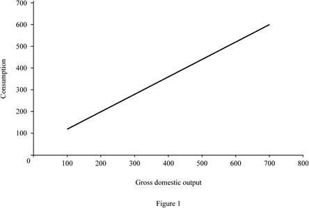
In Figure 1, the horizontal axis measures the gross domestic output and the vertical axis measures the consumption level.
Size of marginal propensity to consume (MPC) can be calculated as follows.
The size of marginal propensity to consume is 0.8.
Concept introduction:
Consumption schedule: Consumption schedule refers to the quantity of consumption at different levels of income.
Marginal propensity to consume (MPS): Marginal propensity to consume refers to the sensitivity of change in the consumption level due to the changes occurred in the income level.
Sub part (b):
Disposable income, tax rate, consumption schedule, marginal propensity to consume and multiplier.
Sub part (b):
Explanation of Solution
Disposable income (DI) can be calculated by using the following formula.
Substitute the respective values in Equation (1) to calculate the disposable income at the level of GDP $100.
Disposable income at the level of GDP $100 is $90.
Tax rate can be calculated by using the following formula.
Substitute the respective values in Equation (2) to calculate the tax rate at the level of GDP $100.
Tax rate at the level of GDP is 10%.
New consumption level can be calculated by using the following formula.
Substitute the respective values in Equation (3) to calculate the disposable income at the level of GDP $100. Since, the tax payment is equal amount of decrease in consumption for all the levels of GDP. The decreasing consumption for increasing $10 is assumed to be $8.
New consumption is $112.
Table -2 shows the values of disposable income, new consumption level after tax and the tax rate that are obtained by using Equations (1), (2) and (3).
Table -2
| Gross domestic product | Tax | DI | New consumption | Tax rate |
| 100 | 10 | 90 | 112 | 10% |
| 200 | 10 | 190 | 192 | 5% |
| 300 | 10 | 290 | 272 | 3.33% |
| 400 | 10 | 390 | 352 | 2.5% |
| 500 | 10 | 490 | 432 | 2% |
| 600 | 10 | 590 | 512 | 1.67% |
| 700 | 10 | 690 | 592 | 1.43% |
Size of marginal propensity to consume (MPC) can be calculated as follows.
The size of marginal propensity to consume is 0.8.
Multiplier: Multiplier refers to the ratio of change in the real GDP to the change in initial consumption, at a constant price rate. Multiplier is positively related to the marginal propensity to consumer and negatively related with the marginal propensity to save. Multiplier can be evaluated using the following formula:
Since the value of MPC remains the same for part (a) and part (b), there is no change in the value of multiplier. The value of multiplier is 5
Figure -2 illustrates the level of consumption at different level of gross domestic product (GDP) for lump sum tax (Regressive tax).
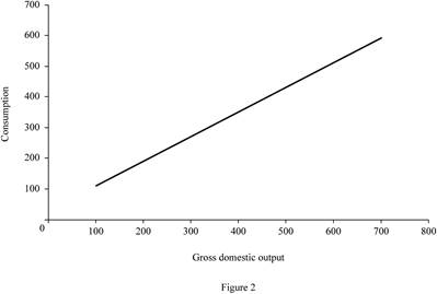
In Figure -2, the horizontal axis measures the gross domestic output and the vertical axis measures the consumption level.
Concept introduction:
Consumption schedule: Consumption schedule refers to the quantity of consumption at different levels of income.
Marginal propensity to consume (MPS): Marginal propensity to consume refers to the sensitivity of change in the consumption level due to the changes occurred in the income level.
Multiplier: Multiplier refers to the ratio of change in the real GDP to the change in initial consumption at constant price rate. Multiplier is positively related to the marginal propensity to consumer and negatively related with the marginal propensity to save.
Sub part (c):
Tax amount, consumption schedule, marginal propensity to consume and multiplier.
Sub part (c):
Explanation of Solution
Tax amount can be calculated by using the following formula.
Substitute the respective values in Equation (4) to calculate the tax amount at $100 GDP.
Tax amount is $10.
Table -3 shows the values of disposable income, new consumption level after tax and the tax rate that are obtained by using Equations (1), (2), (3) and (4). The change in tax amount is differing for different levels of GDP. The decreasing consumption for increasing each $10 is assumed to be $8 (Thus, if the tax payment is $30, then the consumption decreases by $24
Table -3
| Gross domestic product | Tax | DI | New consumption | Tax rate |
| 100 | 10 | 90 | 112 | 10% |
| 200 | 20 | 180 | 184 | 10% |
| 300 | 30 | 270 | 256 | 10% |
| 400 | 40 | 360 | 328 | 10% |
| 500 | 50 | 450 | 400 | 10% |
| 600 | 60 | 540 | 472 | 10% |
| 700 | 70 | 630 | 544 | 10% |
Multiplier: Multiplier refers to the ratio of change in the real GDP to the change in initial consumption, at a constant price rate. Multiplier is positively related to the marginal propensity to consumer and negatively related with the marginal propensity to save. Multiplier can be evaluated using the following formula:
Since the value of MPC different for part (a) and part (c), the value of multiplier for both the part is different. The value of multiplier is 3.57
Figure -3 illustrates the level of consumption at different level of gross domestic product (GDP) for proportional tax.
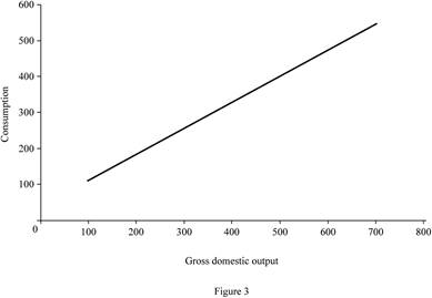
In Figure -3, the horizontal axis measures the gross domestic output and the vertical axis measures the consumption level.
Concept introduction:
Consumption schedule: Consumption schedule refers to the quantity of consumption at different levels of income.
Marginal propensity to consume (MPS): Marginal propensity to consume refers to the sensitivity of change in the consumption level due to the changes occurred in the income level.
Multiplier: Multiplier refers to the ratio of change in the real GDP to the change in initial consumption at constant price rate. Multiplier is positively related to the marginal propensity to consumer and negatively related with the marginal propensity to save.
Sub part (d):
consumption schedule, marginal propensity to consume and multiplier.
Sub part (d):
Explanation of Solution
Marginal propensity to consume can be calculated by using the following formula.
Substitute the respective values in Equation (5) to calculate the MPC at $100 GDP.
The value of MPC is 0.72.
Table -4 shows the values of disposable income, new consumption level after tax and the tax rate that are obtained by using Equations (1), (2), (3), (4) and (5). The change in tax amount is differing for different levels of GDP. The decreasing consumption for increasing each $10 is assumed to be $8 (Thus, if the tax payment is $20, then the consumption decreases by $16
Table -3
| Gross domestic product | Tax | DI | New consumption | Tax rate | MPC |
| 100 | 0 | 100 | 120 | 0% | |
| 200 | 10 | 190 | 192 | 5% | 0.8 |
| 300 | 30 | 270 | 256 | 10% | 0.64 |
| 400 | 60 | 340 | 312 | 15% | 0.56 |
| 500 | 100 | 400 | 360 | 20% | 0.48 |
| 600 | 150 | 450 | 400 | 25% | 0.4 |
| 700 | 210 | 490 | 432 | 30% | 0.32 |
Multiplier: Multiplier refers to the ratio of change in the real GDP to the change in initial consumption, at a constant price rate. Multiplier is positively related to the marginal propensity to consumer and negatively related with the marginal propensity to save.
Multiplier value is differing for each level of GDP. When the tax rate increases, it reduces the value of MPC. Since the value of MPC decreases, the value of multiplier will also decrease.
Figure 4 illustrates the level of consumption at different level of gross domestic product (GDP) for progressive tax.
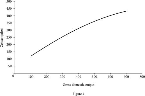
In Figure 4, the horizontal axis measures the gross domestic output and the vertical axis measures the consumption level.
Concept introduction:
Consumption schedule: Consumption schedule refers to the quantity of consumption at different levels of income.
Marginal propensity to consume (MPS): Marginal propensity to consume refers to the sensitivity of change in the consumption level due to the changes occurred in the income level.
Multiplier: Multiplier refers to the ratio of change in the real GDP to the change in initial consumption at constant price rate. Multiplier is positively related to the marginal propensity to consumer and negatively related with the marginal propensity to save.
Sup part (e):
Marginal propensity to consume and multiplier.
Sup part (e):
Explanation of Solution
Figure 1, Figure 2, Figure 3 and Figure 4 reveals that the proportional and progressive tax system reduces the value of MPC, so that the value of multiplier also decreases. The regressive tax system (Lump sum tax) does not alter the MPC. Since there is no change in the MPC, the multiplier remains the same.
Concept introduction:
Marginal propensity to consume (MPS): Marginal propensity to consume refers to the sensitivity of change in the consumption level due to the changes occurred in the income level.
Progressive tax: Progressive tax refers to the higher income people paying higher tax amount than the lower income people.
Proportional tax: Proportional tax rate refers to the fixed tax rate regardless of income and the tax rate and is the same for all levels of income.
Regressive tax: Regressive tax refers to the higher income people paying lower percentage of tax amount and lower income people paying higher percentage of tax amount.
Multiplier: Multiplier refers to the ratio of change in the real GDP to the change in initial consumption at constant price rate. Multiplier is positively related to the marginal propensity to consumer and negatively related with the marginal propensity to save.
Want to see more full solutions like this?

- How does the mining industry in canada contribute to the Canadian economy? Describe why your industry is so important to the Canadian economy What would happen if your industry disappeared, or suffered significant layoffs?arrow_forwardWhat is already being done to make mining in canada more sustainable? What efforts are being made in order to make mining more sustainable?arrow_forwardWhat are the environmental challenges the canadian mining industry face? Discuss current challenges that mining faces with regard to the environmentarrow_forward
- What sustainability efforts have been put forth in the mining industry in canada Are your industry’s resources renewable or non-renewable? How do you know? Describe your industry’s reclamation processarrow_forwardHow does oligopolies practice non-price competition in South Africa?arrow_forwardWhat are the advantages and disadvantages of oligopolies on the consumers, businesses and the economy as a whole?arrow_forward
- 1. After the reopening of borders with mainland China following the COVID-19 lockdown, residents living near the border now have the option to shop for food on either side. In Hong Kong, the cost of food is at its listed price, while across the border in mainland China, the price is only half that of Hong Kong's. A recent report indicates a decline in food sales in Hong Kong post-reopening. ** Diagrams need not be to scale; Focus on accurately representing the relevant concepts and relationships rather than the exact proportions. (a) Using a diagram, explain why Hong Kong's food sales might have dropped after the border reopening. Assume that consumers are indifferent between purchasing food in Hong Kong or mainland China, and therefore, their indifference curves have a slope of one like below. Additionally, consider that there are no transport costs and the daily food budget for consumers is identical whether they shop in Hong Kong or mainland China. I 3. 14 (b) In response to the…arrow_forward2. Health Food Company is a well-known global brand that specializes in healthy and organic food products. One of their main products is organic chicken, which they source from small farmers in the area. Health Food Company is the sole buyer of organic chicken in the market. (a) In the context of the organic chicken industry, what type of market structure is Health Food Company operating in? (b) Using a diagram, explain how the identified market structure affects the input pricing and output decisions of Health Food Company. Specifically, include the relevant curves and any key points such as the profit-maximizing price and quantity. () (c) How can encouraging small chicken farmers to form bargaining associations help improve their trade terms? Explain how this works by drawing on the graph in answer (b) to illustrate your answer.arrow_forward2. Suppose that a farmer has two ways to produce his crop. He can use a low-polluting technology with the marginal cost curve MCL or a high polluting technology with the marginal cost curve MCH. If the farmer uses the high-polluting technology, for each unit of quantity produced, one unit of pollution is also produced. Pollution causes pollution damages that are valued at $E per unit. The good produced can be sold in the market for $P per unit. P 1 MCH 0 Q₁ MCL Q2 E a. b. C. If there are no restrictions on the firm's choices, which technology will the farmer use and what quantity will he produce? Explain, referring to the area identified in the figure Given your response in part a, is it socially efficient for there to be no restriction on production? Explain, referring to the area identified in the figure If the government restricts production to Q1, what technology would the farmer choose? Would a socially efficient outcome be achieved? Explain, referring to the area identified in…arrow_forward
- I need help in seeing how these are the answers. If you could please write down your steps so I can see how it's done please.arrow_forwardSuppose that a random sample of 216 twenty-year-old men is selected from a population and that their heights and weights are recorded. A regression of weight on height yields Weight = (-107.3628) + 4.2552 x Height, R2 = 0.875, SER = 11.0160 (2.3220) (0.3348) where Weight is measured in pounds and Height is measured in inches. A man has a late growth spurt and grows 1.6200 inches over the course of a year. Construct a confidence interval of 90% for the person's weight gain. The 90% confidence interval for the person's weight gain is ( ☐ ☐) (in pounds). (Round your responses to two decimal places.)arrow_forwardSuppose that (Y, X) satisfy the assumptions specified here. A random sample of n = 498 is drawn and yields Ŷ= 6.47 + 5.66X, R2 = 0.83, SER = 5.3 (3.7) (3.4) Where the numbers in parentheses are the standard errors of the estimated coefficients B₁ = 6.47 and B₁ = 5.66 respectively. Suppose you wanted to test that B₁ is zero at the 5% level. That is, Ho: B₁ = 0 vs. H₁: B₁ #0 Report the t-statistic and p-value for this test. Definition The t-statistic is (Round your response to two decimal places) ☑ The Least Squares Assumptions Y=Bo+B₁X+u, i = 1,..., n, where 1. The error term u; has conditional mean zero given X;: E (u;|X;) = 0; 2. (Y;, X¡), i = 1,..., n, are independent and identically distributed (i.i.d.) draws from i their joint distribution; and 3. Large outliers are unlikely: X; and Y, have nonzero finite fourth moments.arrow_forward

 Principles of Economics 2eEconomicsISBN:9781947172364Author:Steven A. Greenlaw; David ShapiroPublisher:OpenStax
 Essentials of Economics (MindTap Course List)EconomicsISBN:9781337091992Author:N. Gregory MankiwPublisher:Cengage Learning
 Brief Principles of Macroeconomics (MindTap Cours...EconomicsISBN:9781337091985Author:N. Gregory MankiwPublisher:Cengage Learning
