
Videos
Note: Exercises marked * are based on optional material.
Instructions for Data Sets: Choose one of the data sets A–K below or as assigned by your instructor. Only the first three and last three observations are shown for each data set. In each data set, the dependent variable (response) is the first variable. Choose the independent variables (predictors) as you judge appropriate. Use a spreadsheet or a statistical package (e.g., MegaStat or Minitab) to perform the necessary regression calculations and to obtain the required graphs. Write a concise report answering questions 13.25 through 13.41 (or a subset of these questions assigned by your instructor). Label sections of your report to correspond to the questions. Insert tables and graphs in your report as appropriate. You may work with a partner if your instructor allows it.
If you did not already do so, request leverage statistics. Are any observations influential? Explain.
Find leverage statistics.
Identify any of the observations are influential.
Answer to Problem 38CE
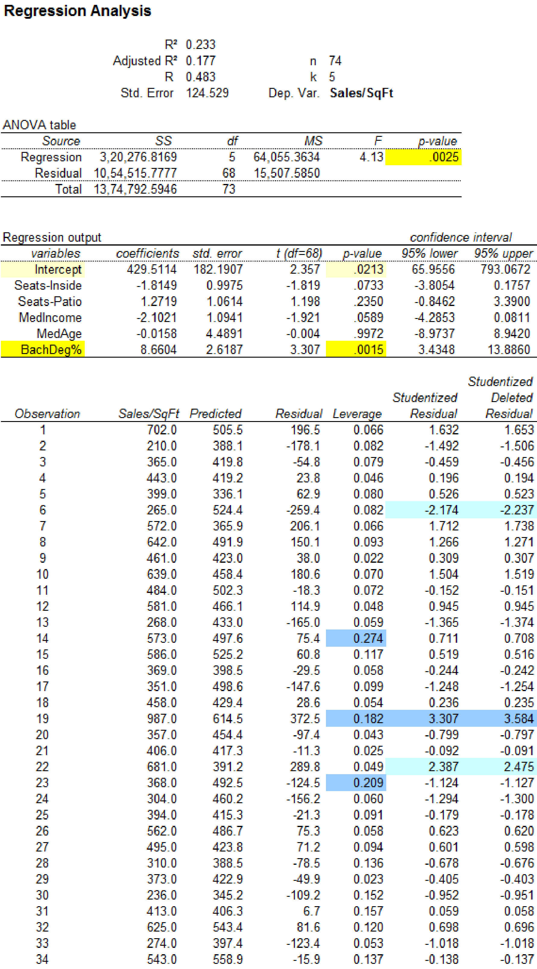
The leverage statistics are,
| Observation | Sales/SqFt | Predicted | Residual | Leverage |
| 1 | 702 | 505.5378 | 196.4622 | 0.0659 |
| 2 | 210 | 388.0933 | –178.093 | 0.0818 |
| 3 | 365 | 419.7986 | –54.7986 | 0.0789 |
| 4 | 443 | 419.2017 | 23.79828 | 0.0458 |
| 5 | 399 | 336.1339 | 62.86605 | 0.0798 |
| 6 | 265 | 524.3932 | –259.393 | 0.0816 |
| 7 | 572 | 365.8614 | 206.1386 | 0.0655 |
| 8 | 642 | 491.9392 | 150.0608 | 0.0935 |
| 9 | 461 | 422.9892 | 38.0108 | 0.0225 |
| 10 | 639 | 458.365 | 180.635 | 0.0703 |
| 11 | 484 | 502.2794 | –18.2794 | 0.0715 |
| 12 | 581 | 466.1341 | 114.8659 | 0.0478 |
| 13 | 268 | 432.9745 | –164.974 | 0.0586 |
| 14 | 573 | 497.5596 | 75.44042 | 0.2737 |
| 15 | 586 | 525.2306 | 60.76944 | 0.1168 |
| 16 | 369 | 398.5007 | –29.5007 | 0.0584 |
| 17 | 351 | 498.6047 | –147.605 | 0.0985 |
| 18 | 458 | 429.3871 | 28.61286 | 0.0535 |
| 19 | 987 | 614.5091 | 372.4909 | 0.1820 |
| 20 | 357 | 454.3592 | –97.3592 | 0.0429 |
| 21 | 406 | 417.2942 | –11.2942 | 0.0250 |
| 22 | 681 | 391.1612 | 289.8388 | 0.0493 |
| 23 | 368 | 492.4983 | –124.498 | 0.2093 |
| 24 | 304 | 460.1672 | –156.167 | 0.0604 |
| 25 | 394 | 415.2689 | –21.2689 | 0.0913 |
| 26 | 562 | 486.68 | 75.31997 | 0.0580 |
| 27 | 495 | 423.7816 | 71.21836 | 0.0942 |
| 28 | 310 | 388.496 | –78.496 | 0.1363 |
| 29 | 373 | 422.8679 | –49.8679 | 0.0227 |
| 30 | 236 | 345.16 | –109.16 | 0.1516 |
| 31 | 413 | 406.2904 | 6.709589 | 0.1565 |
| 32 | 625 | 543.4075 | 81.59252 | 0.1197 |
| 33 | 274 | 397.4102 | –123.41 | 0.0526 |
| 34 | 543 | 558.9323 | –15.9323 | 0.1372 |
| 35 | 179 | 297.105 | –118.105 | 0.0794 |
| 36 | 375 | 361.7308 | 13.26922 | 0.0837 |
| 37 | 329 | 433.9038 | –104.904 | 0.0659 |
| 38 | 297 | 430.0182 | –133.018 | 0.0682 |
| 39 | 323 | 455.7566 | –132.757 | 0.0800 |
| 40 | 469 | 404.899 | 64.101 | 0.0291 |
| 41 | 353 | 497.4495 | –144.449 | 0.0837 |
| 42 | 380 | 491.0586 | –111.059 | 0.0696 |
| 43 | 398 | 408.7628 | –10.7628 | 0.0353 |
| 44 | 312 | 318.6083 | –6.60827 | 0.0574 |
| 45 | 452 | 432.4409 | 19.55915 | 0.0731 |
| 46 | 699 | 362.4679 | 336.5321 | 0.0617 |
| 47 | 367 | 347.5704 | 19.42961 | 0.0801 |
| 48 | 432 | 380.8856 | 51.11438 | 0.0736 |
| 49 | 367 | 355.4863 | 11.51368 | 0.0922 |
| 50 | 401 | 381.559 | 19.44102 | 0.0432 |
| 51 | 414 | 481.2256 | –67.2256 | 0.0375 |
| 52 | 481 | 428.1006 | 52.89939 | 0.0183 |
| 53 | 538 | 415.7548 | 122.2452 | 0.0271 |
| 54 | 330 | 359.279 | –29.279 | 0.0356 |
| 55 | 250 | 438.5112 | –188.511 | 0.0532 |
| 56 | 292 | 396.9591 | –104.959 | 0.0582 |
| 57 | 517 | 411.7635 | 105.2365 | 0.0231 |
| 58 | 552 | 470.1005 | 81.89945 | 0.0275 |
| 59 | 387 | 361.7699 | 25.23009 | 0.0832 |
| 60 | 427 | 408.3022 | 18.69777 | 0.0631 |
| 61 | 454 | 497.6884 | –43.6884 | 0.0887 |
| 62 | 512 | 441.1052 | 70.89483 | 0.0793 |
| 63 | 345 | 375.7731 | –30.7731 | 0.1071 |
| 64 | 234 | 334.17 | –100.17 | 0.0622 |
| 65 | 348 | 333.4539 | 14.54613 | 0.1051 |
| 66 | 348 | 458.6665 | –110.666 | 0.1285 |
| 67 | 295 | 315.655 | –20.655 | 0.1077 |
| 68 | 361 | 376.5859 | –15.5859 | 0.0450 |
| 69 | 468 | 232.9942 | 235.0058 | 0.2319 |
| 70 | 404 | 393.7594 | 10.24059 | 0.1052 |
| 71 | 246 | 373.6202 | –127.62 | 0.1022 |
| 72 | 340 | 403.9505 | –63.9505 | 0.1144 |
| 73 | 401 | 413.2786 | –12.2786 | 0.0619 |
| 74 | 327 | 316.5622 | 10.43785 | 0.1045 |
The observations 14, 19, 23 and 69 are considered to have higher leverage values.
The influential observation is 23.
Explanation of Solution
Calculation
The given information is that, the dataset of ‘Noodles & Company Sales, Seating, and Demographic data’ contains
Software procedure:
Step by step procedure to obtain regression output using MegaStat software is given as,
- • Choose MegaStat >Correlation/Regression>Regression Analysis.
- • SelectInput ranges, enter the variable range for ‘Seats-Inside, Seats-Patio, MedIncome, MedAge, BachDeg%’ as the column of X, Independent variable(s)
- • Enter the variable range for ‘Sales/SqFt’ as the column of Y, Dependent variable.
- • In Options> Residuals chooseDiagnostics and influential residuals.
- • Click OK.
Output using MegaStatsoftware is given below:
Influential observation:
The influential observation has a great effect on the parameters of the regression line when it is removed from the data set.
The influential observations can be identified using the leverage values. If the observation have the high leverage value, that is any leverage statistic is greater than value of
Substitute,
The leverage statistics greater than 0.1622 are, 0.274 corresponding to observation 14, 0.182 corresponding to observation 19, 0.209 corresponding to observation 23 and 0.232 corresponding to observation 69
The observations 14, 19, 23 and 69 are considered to have higher leverage values.
Regression conclusion including all observations:
Let
The p-value for predictor seats-inside is 0.0733.
The p-value for predictor seats-patio is 0.2350.
The p-value for predictor MedIncome is 0.0589.
The p-value for predictor MedAge is 0.9972.
The p-value for predictor BachDeg% is 0.0015.
Null hypothesis:
The predictor variable j is not related to annual sales.
Alternative hypothesis:
The predictor variable j is related to annual sales.
Rejection rules:
- • If p-value is less than the level of significance then the null hypothesis is rejected. The predictor is significant.
- • If p-value is greater than the level of significance then the null hypothesis is not rejected. The predictor is not significant.
Conclusion for seats-inside:
The p-value for predictor seats-inside is 0.0733.
The level of significance is 0.05.
The p-value is greater than the level of significance.
That is,
The null hypothesis is not rejected.
The predictor variable seats-inside is not related to annual sales.
The predictor seats-inside is not significant.
Conclusion for seats-patio:
The p-value for predictor seats-patio is 0.2350.
The level of significance is 0.05.
The p-value is greater than the level of significance.
That is,
The null hypothesis is not rejected.
The predictor variable seats-patio is not related to annual sales.
The predictor seats-patio is not significant.
Conclusion for median income:
The p-value for predictor median income is 0.0589.
The level of significance is 0.05.
The p-value is greater than the level of significance.
That is,
The null hypothesis is not rejected.
The predictor variable median income is not related to annual sales.
The predictor median income is not significant.
Conclusion for median age:
The p-value for predictor median age of population is 0.9972.
The level of significance is 0.05.
The p-value is greater than the level of significance.
That is,
The null hypothesis is not rejected.
The predictor variable median age of population is not related to annual sales.
The predictor median age of population is not significant.
Conclusion for ‘% with Bachelor's Degree’:
The p-value for predictor ‘% with Bachelor's Degree’ is 0.0015.
The level of significance is 0.05.
The p-value is less than the level of significance.
That is,
The null hypothesis is rejected.
The predictor variable ‘% with Bachelor's Degree’ is related to annual sales.
The predictor ‘% with Bachelor's Degree’of population is significant.
The p-value for ‘% with Bachelor's Degree’ indicates predictor significance at
Regression analysis by removing the observation 14:
Software procedure:
Step by step procedure to obtain regression equation using MegaStat software is given as,
- • Choose MegaStat >Correlation/Regression>Regression Analysis.
- • SelectInput ranges, enter the variable range for ‘Seats-Inside, Seats-Patio, MedIncome, MedAge, BachDeg%’ as the column of X, Independent variable(s)
- • Enter the variable range for ‘Sales/SqFt’ as the column of Y, Dependent variable.
- • Click OK.
Output using MegaStatsoftware is given below:
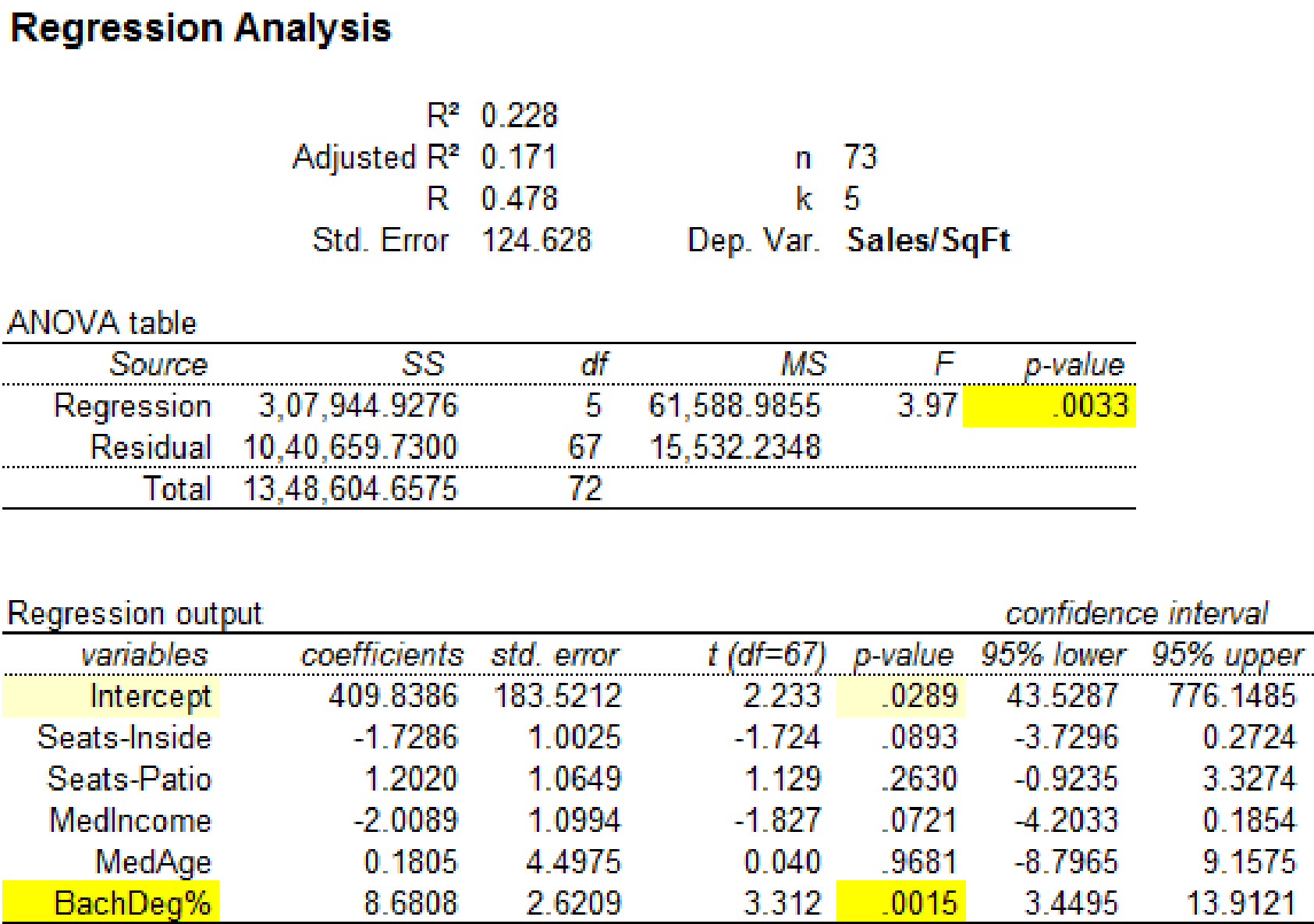
It is clear that the predictor variable ‘BachDeg%’ with p-value 0.0015 is significant at
Regression analysis by removing the observation 19:
Software procedure:
Step by step procedure to obtain regression equation using MegaStat software is given as,
- • Choose MegaStat >Correlation/Regression>Regression Analysis.
- • SelectInput ranges, enter the variable range for ‘Seats-Inside, Seats-Patio, MedIncome, MedAge, BachDeg%’ as the column of X, Independent variable(s)
- • Enter the variable range for ‘Sales/SqFt’ as the column of Y, Dependent variable.
- • Click OK.
Output using MegaStatsoftware is given below:
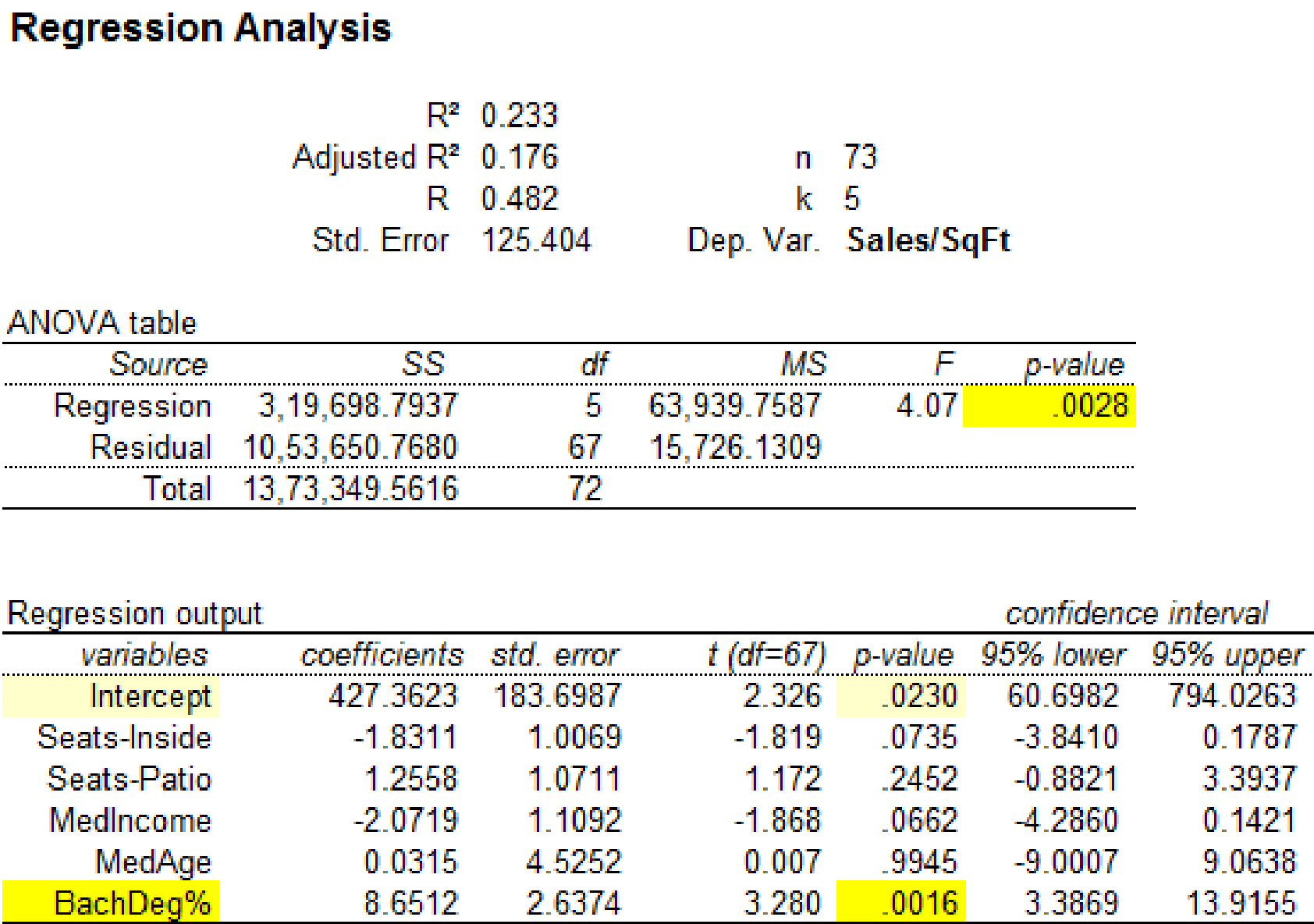
It is clear that the predictor variable ‘BachDeg%’ with p-value 0.0016 is significant at
Regression analysis by removing the observation 23:
Software procedure:
Step by step procedure to obtain regression equation using MegaStat software is given as,
- • Choose MegaStat >Correlation/Regression>Regression Analysis.
- • SelectInput ranges, enter the variable range for ‘Seats-Inside, Seats-Patio, MedIncome, MedAge, BachDeg%’ as the column of X, Independent variable(s)
- • Enter the variable range for ‘Sales/SqFt’ as the column of Y, Dependent variable.
- • Click OK.
Output using MegaStatsoftware is given below:
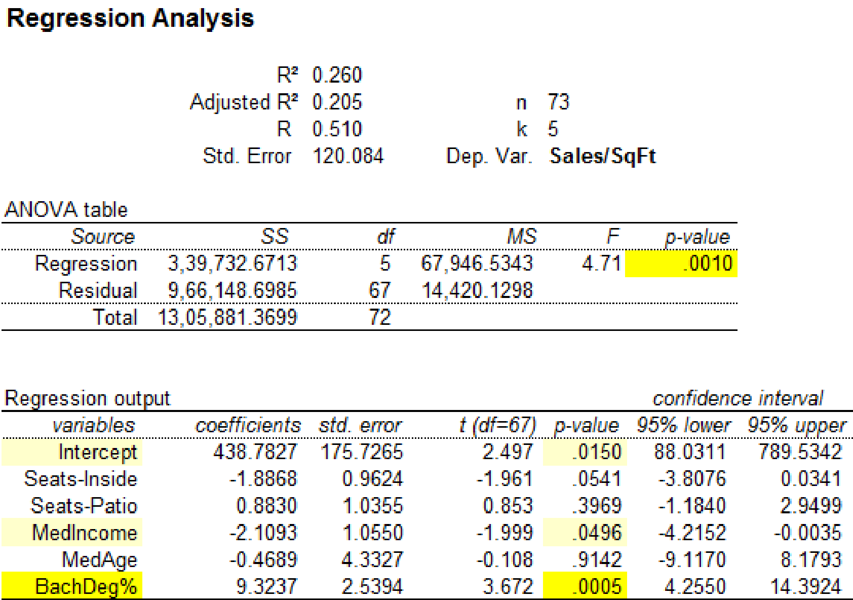
It is clear that the predictor variables ‘MedIncome’ with p-value 0.0496 and ‘BachDeg%’ with p-value 0.0016 are significant at
Regression analysis by removing the observation 69:
Software procedure:
Step by step procedure to obtain regression equation using MegaStat software is given as,
- • Choose MegaStat >Correlation/Regression>Regression Analysis.
- • SelectInput ranges, enter the variable range for ‘Seats-Inside, Seats-Patio, MedIncome, MedAge, BachDeg%’ as the column of X, Independent variable(s)
- • Enter the variable range for ‘Sales/SqFt’ as the column of Y, Dependent variable.
- • Click OK.
Output using MegaStatsoftware is given below:
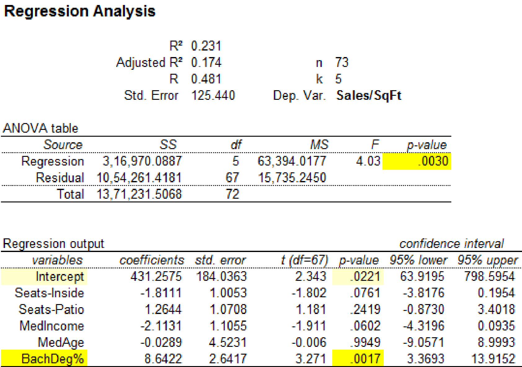
It is clear that the predictor variable ‘BachDeg%’ with p-value 0.0017 is significant at
The significance for the regression statistics has changed when the observation 23 is removed from the data set. Hence, the influential observation is 23.
Want to see more full solutions like this?
Chapter 13 Solutions
Gen Combo Ll Applied Statistics In Business & Economics; Connect Access Card


- The accompanying data shows the fossil fuels production, fossil fuels consumption, and total energy consumption in quadrillions of BTUs of a certain region for the years 1986 to 2015. Complete parts a and b. Year Fossil Fuels Production Fossil Fuels Consumption Total Energy Consumption1949 28.748 29.002 31.9821950 32.563 31.632 34.6161951 35.792 34.008 36.9741952 34.977 33.800 36.7481953 35.349 34.826 37.6641954 33.764 33.877 36.6391955 37.364 37.410 40.2081956 39.771 38.888 41.7541957 40.133 38.926 41.7871958 37.216 38.717 41.6451959 39.045 40.550 43.4661960 39.869 42.137 45.0861961 40.307 42.758 45.7381962 41.732 44.681 47.8261963 44.037 46.509 49.6441964 45.789 48.543 51.8151965 47.235 50.577 54.0151966 50.035 53.514 57.0141967 52.597 55.127 58.9051968 54.306 58.502 62.4151969 56.286…arrow_forwardThe accompanying data shows the fossil fuels production, fossil fuels consumption, and total energy consumption in quadrillions of BTUs of a certain region for the years 1986 to 2015. Complete parts a and b. Year Fossil Fuels Production Fossil Fuels Consumption Total Energy Consumption1949 28.748 29.002 31.9821950 32.563 31.632 34.6161951 35.792 34.008 36.9741952 34.977 33.800 36.7481953 35.349 34.826 37.6641954 33.764 33.877 36.6391955 37.364 37.410 40.2081956 39.771 38.888 41.7541957 40.133 38.926 41.7871958 37.216 38.717 41.6451959 39.045 40.550 43.4661960 39.869 42.137 45.0861961 40.307 42.758 45.7381962 41.732 44.681 47.8261963 44.037 46.509 49.6441964 45.789 48.543 51.8151965 47.235 50.577 54.0151966 50.035 53.514 57.0141967 52.597 55.127 58.9051968 54.306 58.502 62.4151969 56.286…arrow_forwardThe accompanying data shows the fossil fuels production, fossil fuels consumption, and total energy consumption in quadrillions of BTUs of a certain region for the years 1986 to 2015. Complete parts a and b. Develop line charts for each variable and identify the characteristics of the time series (that is, random, stationary, trend, seasonal, or cyclical). What is the line chart for the variable Fossil Fuels Production?arrow_forward
- The accompanying data shows the fossil fuels production, fossil fuels consumption, and total energy consumption in quadrillions of BTUs of a certain region for the years 1986 to 2015. Complete parts a and b. Year Fossil Fuels Production Fossil Fuels Consumption Total Energy Consumption1949 28.748 29.002 31.9821950 32.563 31.632 34.6161951 35.792 34.008 36.9741952 34.977 33.800 36.7481953 35.349 34.826 37.6641954 33.764 33.877 36.6391955 37.364 37.410 40.2081956 39.771 38.888 41.7541957 40.133 38.926 41.7871958 37.216 38.717 41.6451959 39.045 40.550 43.4661960 39.869 42.137 45.0861961 40.307 42.758 45.7381962 41.732 44.681 47.8261963 44.037 46.509 49.6441964 45.789 48.543 51.8151965 47.235 50.577 54.0151966 50.035 53.514 57.0141967 52.597 55.127 58.9051968 54.306 58.502 62.4151969 56.286…arrow_forwardFor each of the time series, construct a line chart of the data and identify the characteristics of the time series (that is, random, stationary, trend, seasonal, or cyclical). Month PercentApr 1972 4.97May 1972 5.00Jun 1972 5.04Jul 1972 5.25Aug 1972 5.27Sep 1972 5.50Oct 1972 5.73Nov 1972 5.75Dec 1972 5.79Jan 1973 6.00Feb 1973 6.02Mar 1973 6.30Apr 1973 6.61May 1973 7.01Jun 1973 7.49Jul 1973 8.30Aug 1973 9.23Sep 1973 9.86Oct 1973 9.94Nov 1973 9.75Dec 1973 9.75Jan 1974 9.73Feb 1974 9.21Mar 1974 8.85Apr 1974 10.02May 1974 11.25Jun 1974 11.54Jul 1974 11.97Aug 1974 12.00Sep 1974 12.00Oct 1974 11.68Nov 1974 10.83Dec 1974 10.50Jan 1975 10.05Feb 1975 8.96Mar 1975 7.93Apr 1975 7.50May 1975 7.40Jun 1975 7.07Jul 1975 7.15Aug 1975 7.66Sep 1975 7.88Oct 1975 7.96Nov 1975 7.53Dec 1975 7.26Jan 1976 7.00Feb 1976 6.75Mar 1976 6.75Apr 1976 6.75May 1976…arrow_forwardHi, I need to make sure I have drafted a thorough analysis, so please answer the following questions. Based on the data in the attached image, develop a regression model to forecast the average sales of football magazines for each of the seven home games in the upcoming season (Year 10). That is, you should construct a single regression model and use it to estimate the average demand for the seven home games in Year 10. In addition to the variables provided, you may create new variables based on these variables or based on observations of your analysis. Be sure to provide a thorough analysis of your final model (residual diagnostics) and provide assessments of its accuracy. What insights are available based on your regression model?arrow_forward
- I want to make sure that I included all possible variables and observations. There is a considerable amount of data in the images below, but not all of it may be useful for your purposes. Are there variables contained in the file that you would exclude from a forecast model to determine football magazine sales in Year 10? If so, why? Are there particular observations of football magazine sales from previous years that you would exclude from your forecasting model? If so, why?arrow_forwardStat questionsarrow_forward1) and let Xt is stochastic process with WSS and Rxlt t+t) 1) E (X5) = \ 1 2 Show that E (X5 = X 3 = 2 (= = =) Since X is WSSEL 2 3) find E(X5+ X3)² 4) sind E(X5+X2) J=1 ***arrow_forward
- Prove that 1) | RxX (T) | << = (R₁ " + R$) 2) find Laplalse trans. of Normal dis: 3) Prove thy t /Rx (z) | < | Rx (0)\ 4) show that evary algebra is algebra or not.arrow_forwardFor each of the time series, construct a line chart of the data and identify the characteristics of the time series (that is, random, stationary, trend, seasonal, or cyclical). Month Number (Thousands)Dec 1991 65.60Jan 1992 71.60Feb 1992 78.80Mar 1992 111.60Apr 1992 107.60May 1992 115.20Jun 1992 117.80Jul 1992 106.20Aug 1992 109.90Sep 1992 106.00Oct 1992 111.80Nov 1992 84.50Dec 1992 78.60Jan 1993 70.50Feb 1993 74.60Mar 1993 95.50Apr 1993 117.80May 1993 120.90Jun 1993 128.50Jul 1993 115.30Aug 1993 121.80Sep 1993 118.50Oct 1993 123.30Nov 1993 102.30Dec 1993 98.70Jan 1994 76.20Feb 1994 83.50Mar 1994 134.30Apr 1994 137.60May 1994 148.80Jun 1994 136.40Jul 1994 127.80Aug 1994 139.80Sep 1994 130.10Oct 1994 130.60Nov 1994 113.40Dec 1994 98.50Jan 1995 84.50Feb 1995 81.60Mar 1995 103.80Apr 1995 116.90May 1995 130.50Jun 1995 123.40Jul 1995 129.10Aug 1995…arrow_forwardFor each of the time series, construct a line chart of the data and identify the characteristics of the time series (that is, random, stationary, trend, seasonal, or cyclical). Year Month Units1 Nov 42,1611 Dec 44,1862 Jan 42,2272 Feb 45,4222 Mar 54,0752 Apr 50,9262 May 53,5722 Jun 54,9202 Jul 54,4492 Aug 56,0792 Sep 52,1772 Oct 50,0872 Nov 48,5132 Dec 49,2783 Jan 48,1343 Feb 54,8873 Mar 61,0643 Apr 53,3503 May 59,4673 Jun 59,3703 Jul 55,0883 Aug 59,3493 Sep 54,4723 Oct 53,164arrow_forward
 Holt Mcdougal Larson Pre-algebra: Student Edition...AlgebraISBN:9780547587776Author:HOLT MCDOUGALPublisher:HOLT MCDOUGAL
 Glencoe Algebra 1, Student Edition, 9780079039897...AlgebraISBN:9780079039897Author:CarterPublisher:McGraw Hill
 Big Ideas Math A Bridge To Success Algebra 1: Stu...AlgebraISBN:9781680331141Author:HOUGHTON MIFFLIN HARCOURTPublisher:Houghton Mifflin Harcourt
 Functions and Change: A Modeling Approach to Coll...AlgebraISBN:9781337111348Author:Bruce Crauder, Benny Evans, Alan NoellPublisher:Cengage Learning