Subpart (a):
Marginal revenue.
Subpart (a):
Explanation of Solution
In case A, part (I):
Marginal revenue equation can be derived as follows:
Marginal revenue equation is 50-2Q.
When the quantity is 0 units, the marginal revenue can be calculated by substituting the respective values in the marginal revenue equation.
Marginal revenue is 50 at the point where the quantity is 0 units.
When the quantity is 25 units, the marginal revenue can be calculated by substituting the respective values in the marginal revenue equation.
Marginal revenue is 0 at the point where the quantity is 50 units.
Figure 1 illustrates the marginal revenue curve for 50-2Q.
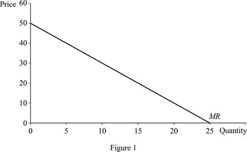
In Figure 1, the vertical axis measures price and the horizontal axis measures quantity; when the quantity is zero, the price would be 50. At price zero, the quantity demanded is 25; thus, this joins the two points the marginal revenue curve gets.
In case A, part (II):
The profit-maximizing output can be calculated by equating the marginal revenue to the marginal cost. This can be done as follows:
Profit-maximizing output is 20 units.
In case A, part (III):
Substitute the profit-maximizing output in the
Profit-maximizing price is $30.
In case A, part (IV):
Total revenue can be obtained by multiplying the profit-maximizing price with the profit-maximizing quantity. This can be done as follows:
Total revenue is $600.
Total cost can be calculated as follows:
Total cost is $300.
In case A, part (V):
Profit can be calculated as follows:
Profit is $300.
In case B, part (I):
Marginal revenue equation can be derived as follows:
Marginal revenue equation is 100-4Q.
When quantity is 0 units, the marginal revenue can be calculated by substituting the respective values in the marginal revenue equation.
Marginal revenue is 100 at the point where the quantity is 0 units.
When quantity is 25 units, the marginal revenue can be calculated by substituting the respective values in the marginal revenue equation.
Marginal revenue is 0 at the point where the quantity is 50 units.
Figure 2 illustrates the marginal revenue curve for 100-4Q.
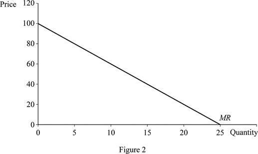
In Figure 2, the vertical axis measures price and the horizontal axis measures quantity. When the quantity is zero, the price would be 100, and at price zero, the quantity demanded is 25. Thus, joining the two points can help obtain the marginal revenue curve.
In case B, part (II):
Profit-maximizing output can be calculated by equating the marginal revenue to the marginal cost. This can be done as follows:
Profit-maximizing output is 22.5 units.
In case B, part (III):
Substitute the profit-maximizing output in the demand equation to calculate the profit maximizing price.
Profit-maximizing price is $55.
In case B, part (IV):
Total revenue can be obtained by multiplying the profit-maximizing price with profit-maximizing quantity. This can be done as follows:
Total revenue is $1,237.5.
Total cost can be calculated as follows:
Total cost is $325.
In case B, part (V):
Profit can be calculated as follows:
Profit is $912.5.
In case C, part (I):
Marginal revenue equation can be derived as follows:
Marginal revenue equation is 100-4Q.
When the quantity is 0 units, the marginal revenue can be calculated by substituting the respective values in the marginal revenue equation.
Marginal revenue is 100 at the point where the quantity is 0 units.
When the quantity is 25 units, the marginal revenue can be calculated by substituting the respective values in the marginal revenue equation.
Marginal revenue is 0 at the point where the quantity is 50 units.
Figure 3 illustrates the marginal revenue curve for100-4Q.
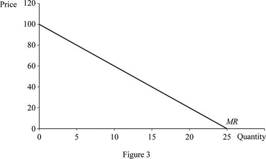
In Figure 3, the vertical axis measures price and the horizontal axis measures quantity. When the quantity is zero, the price would be 100, and at price zero, the quantity demanded is 25. Thus, joining the two points can help obtain the marginal revenue curve.
In case C, part (II):
Profit-maximizing output can be calculated by equating marginal revenue to the marginal cost. This can be done as follows:
Profit-maximizing output is 20 units.
In case C, part (III):
Substitute the profit-maximizing output in demand equation to calculate the profit-maximizing price.
Profit-maximizing price is $60.
In case C, part (IV):
Total revenue can be obtained by multiplying the profit-maximizing price with profit-maximizing quantity. This can be done as follows:
Total revenue is $1,200.
Total cost can be calculated as follows:
Total cost is $500.
In case C, part (V):
Profit can be calculated as follows:
Profit is $700.
Concept introduction:
Marginal revenue: The change in total revenue from selling an additional unit is known as marginal revenue.
Mark-up: Mark-up refers to the amount that is added by the seller to the cost of the goods to determine the selling price.
Sub part (b):
Marginal revenue.
Sub part (b):
Explanation of Solution
The markup refers to the amount that is added by the seller to the cost of the goods to determine the selling price. For calculating the percentage markup, the following equation can be used:
Case A:
Using equation (1), the percentage mark-up in case A can be calculated as follows:
The percentage mark-up in price $20 is 200%.
Case B:
To calculate the percentage mark-up in case B, substitute the values in equation (1).
The percentage mark-up in price $45 is 450%.
Case C:
To calculate the percentage mark-up in case C, substitute the values in equation (1).
The percentage mark-up in price $40 is 200%.
Concept introduction:
Marginal revenue: The change in total revenue from selling an additional unit is known as marginal revenue.
Mark-up: Mark-up refers to the amount that is added by the seller to the cost of the goods to determine the selling price.
Sub part (c):
Marginal revenue.
Sub part (c):
Explanation of Solution
If
Want to see more full solutions like this?
Chapter 13 Solutions
Loose-leaf Version for Modern Principles of Microeconomics & LaunchPad (Six Month Access)

- In a small open economy with a floating exchange rate, the supply of real money balances is fixed and a rise in government spending ______ Group of answer choices Raises the interest rate so that net exports must fall to maintain equilibrium in the goods market. Cannot change the interest rate so that net exports must fall to maintain equilibrium in the goods market. Cannot change the interest rate so income must rise to maintain equilibrium in the money market Raises the interest rate, so that income must rise to maintain equilibrium in the money market.arrow_forwardSuppose a country with a fixed exchange rate decides to implement a devaluation of its currency and commits to maintaining the new fixed parity. This implies (A) ______________ in the demand for its goods and a monetary (B) _______________. Group of answer choices (A) expansion ; (B) contraction (A) contraction ; (B) expansion (A) expansion ; (B) expansion (A) contraction ; (B) contractionarrow_forwardAssume a small open country under fixed exchanges rate and full capital mobility. Prices are fixed in the short run and equilibrium is given initially at point A. An exogenous increase in public spending shifts the IS curve to IS'. Which of the following statements is true? Group of answer choices A new equilibrium is reached at point B. The TR curve will shift down until it passes through point B. A new equilibrium is reached at point C. Point B can only be reached in the absence of capital mobility.arrow_forward
- A decrease in money demand causes the real interest rate to _____ and output to _____ in the short run, before prices adjust to restore equilibrium. Group of answer choices rise; rise fall; fall fall; rise rise; fallarrow_forwardIf a country's policy makers were to continously use expansionary monetary policy in an attempt to hold unemployment below the natural rate , the long urn result would be? Group of answer choices a decrease in the unemployment rate an increase in the level of output All of these an increase in the rate of inflationarrow_forwardA shift in the Aggregate Supply curve to the right will result in a move to a point that is southwest of where the economy is currently at. Group of answer choices True Falsearrow_forward
- An oil shock can cause stagflation, a period of higher inflation and higher unemployment. When this happens, the economy moves to a point to the northeast of where it currently is. After the economy has moved to the northeast, the Federal Reserve can reduce that inflation without having to worry about causing more unemployment. Group of answer choices True Falsearrow_forwardThe long-run Phillips Curve is vertical which indicates Group of answer choices that in the long-run, there is no tradeoff between inflation and unemployment. that in the long-run, there is no tradeoff between inflation and the price level. None of these that in the long-run, the economy returns to a 4 percent level of inflation.arrow_forwardSuppose the exchange rate between the British pound and the U.S. dollar is £1 = $2.00. The U.S. government implementsU.S. government implements a contractionary fiscal policya contractionary fiscal policy. Illustrate the impact of this change in the market for pounds. 1.) Using the line drawing tool, draw and label a new demand line. 2.) Using the line drawing tool, draw and label a new supply line. Note: Carefully follow the instructions above and only draw the required objects.arrow_forward
- Just Part D please, this is for environmental economicsarrow_forward3. Consider a single firm that manufactures chemicals and generates pollution through its emissions E. Researchers have estimated the MDF and MAC curves for the emissions to be the following: MDF = 4E and MAC = 125 – E Policymakers have decided to implement an emissions tax to control pollution. They are aware that a constant per-unit tax of $100 is an efficient policy. Yet they are also aware that this policy is not politically feasible because of the large tax burden it places on the firm. As a result, policymakers propose a two- part tax: a per unit tax of $75 for the first 15 units of emissions an increase in the per unit tax to $100 for all further units of emissions With an emissions tax, what is the general condition that determines how much pollution the regulated party will emit? What is the efficient level of emissions given the above MDF and MAC curves? What are the firm's total tax payments under the constant $100 per-unit tax? What is the firm's total cost of compliance…arrow_forward2. Answer the following questions as they relate to a fishery: Why is the maximum sustainable yield not necessarily the optimal sustainable yield? Does the same intuition apply to Nathaniel's decision of when to cut his trees? What condition will hold at the equilibrium level of fishing in an open-access fishery? Use a graph to explain your answer, and show the level of fishing effort. Would this same condition hold if there was only one boat in the fishery? If not, what condition will hold, and why is it different? Use the same graph to show the single boat's level of effort. Suppose you are given authority to solve the open-access problem in the fishery. What is the key problem that you must address with your policy?arrow_forward

 Principles of Economics (12th Edition)EconomicsISBN:9780134078779Author:Karl E. Case, Ray C. Fair, Sharon E. OsterPublisher:PEARSON
 Engineering Economy (17th Edition)EconomicsISBN:9780134870069Author:William G. Sullivan, Elin M. Wicks, C. Patrick KoellingPublisher:PEARSON
 Principles of Economics (MindTap Course List)EconomicsISBN:9781305585126Author:N. Gregory MankiwPublisher:Cengage Learning
 Managerial Economics: A Problem Solving ApproachEconomicsISBN:9781337106665Author:Luke M. Froeb, Brian T. McCann, Michael R. Ward, Mike ShorPublisher:Cengage Learning
 Managerial Economics & Business Strategy (Mcgraw-...EconomicsISBN:9781259290619Author:Michael Baye, Jeff PrincePublisher:McGraw-Hill Education