
Videos
(a)
To graph: The interaction plot displaying systolic blood pressure on the y-axis and training level on the x-axis.
(a)
Explanation of Solution
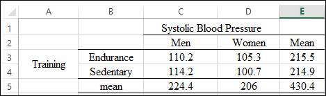
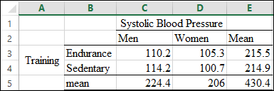
Graph: The problem compares two factors systolic blood pressure on y-axis with training level on x-axis. The factor systolic blood pressure is further classified for men and women and the other factor training level is classified to endurance trained and sedentary men and women. Thus, the table is created for the means of two factor as shown below;
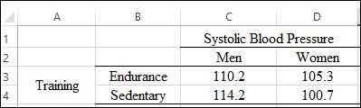
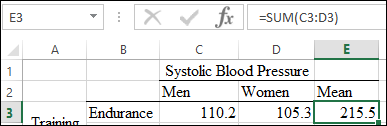
The marginal means for Endurance is calculated by using the
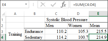
The marginal means for Sedentary is calculated by using the function
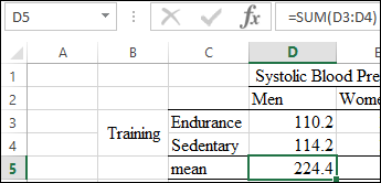
The marginal means for Systolic blood pressure for men is calculated by using the function
The marginal means for Systolic blood pressure for women is calculated by using the function
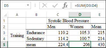
The table is obtained as:
The interaction plot is drawn by following these steps:
Step 1: Open Excel sheet and write the data value. The screenshot is shown below:
Step 2: INSERT>Recommended Charts>All Charts>Line Chart. The screenshot is shown below:

The interaction plot is obtained as shown below:
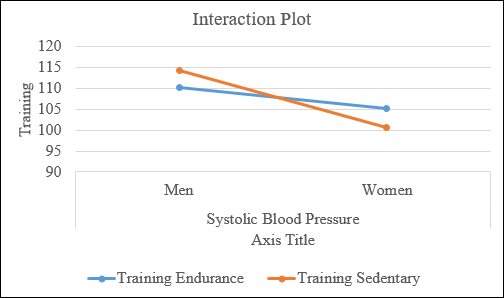
Interpretation: From the chart above, the two lines are not parallel, hence, there is an interaction present between two factors. There is a main effect of training level, training sedentary takes much lower value for women when compared to training endurance for women.
(b)
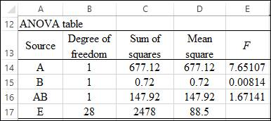
To find: The ANOVA table.
(b)
Answer to Problem 18E
Solution: The ANOVA table is obtained as:
Explanation of Solution
Given: The following values of the Sum of Squares is provided,
where A is the sex effect and B is the training level.
Calculation: The ANOVA table is obtained by following these steps:
Step 1: The degree of freedom for “A” is obtained as follows:
The degree of freedom for “B” is obtained as follows;
The degree of freedom for “AB” is obtained as follows:
The degree of freedom for “E” is obtained as follows:
Step 2: The
The mean squares for “B” is obtained as follows:
The mean squares for “AB” is obtained as follows:
The mean squares for “E” is obtained as follows:
Step 3: The F-value for “A” is obtained as follows:
The F-value for “B” is obtained as follows:
The F-value for “AB” is obtained as follows:
To test the hypothesis for the obtained F-values, the F-critical value is obtained through the F-distribution table as
Interpretation: The comparisons of F-values with F-critical are as follows:
The value of FA is greater than F-critical; hence, the null hypothesis can be rejected significantly, which states that there is a main effect of training level. While the other factor systolic blood pressure and the interaction of these two factors have F-value less than F-critical, which means that they do not show the significant difference in means.
(c)
The benefit of considering pretest measurement.
(c)
Answer to Problem 18E
Solution: It increases the power of the test statistic.
Explanation of Solution
Want to see more full solutions like this?
Chapter 13 Solutions
Introduction to the Practice of Statistics: w/CrunchIt/EESEE Access Card


- Problem 4. Margrabe formula and the Greeks (20 pts) In the homework, we determined the Margrabe formula for the price of an option allowing you to swap an x-stock for a y-stock at time T. For stocks with initial values xo, yo, common volatility σ and correlation p, the formula was given by Fo=yo (d+)-x0Þ(d_), where In (±² Ꭲ d+ õ√T and σ = σ√√√2(1 - p). дго (a) We want to determine a "Greek" for ỡ on the option: find a formula for θα (b) Is дго θα positive or negative? (c) We consider a situation in which the correlation p between the two stocks increases: what can you say about the price Fo? (d) Assume that yo< xo and p = 1. What is the price of the option?arrow_forwardWe consider a 4-dimensional stock price model given (under P) by dẴ₁ = µ· Xt dt + йt · ΣdŴt where (W) is an n-dimensional Brownian motion, π = (0.02, 0.01, -0.02, 0.05), 0.2 0 0 0 0.3 0.4 0 0 Σ= -0.1 -4a За 0 0.2 0.4 -0.1 0.2) and a E R. We assume that ☑0 = (1, 1, 1, 1) and that the interest rate on the market is r = 0.02. (a) Give a condition on a that would make stock #3 be the one with largest volatility. (b) Find the diversification coefficient for this portfolio as a function of a. (c) Determine the maximum diversification coefficient d that you could reach by varying the value of a? 2arrow_forwardQuestion 1. Your manager asks you to explain why the Black-Scholes model may be inappro- priate for pricing options in practice. Give one reason that would substantiate this claim? Question 2. We consider stock #1 and stock #2 in the model of Problem 2. Your manager asks you to pick only one of them to invest in based on the model provided. Which one do you choose and why ? Question 3. Let (St) to be an asset modeled by the Black-Scholes SDE. Let Ft be the price at time t of a European put with maturity T and strike price K. Then, the discounted option price process (ert Ft) t20 is a martingale. True or False? (Explain your answer.) Question 4. You are considering pricing an American put option using a Black-Scholes model for the underlying stock. An explicit formula for the price doesn't exist. In just a few words (no more than 2 sentences), explain how you would proceed to price it. Question 5. We model a short rate with a Ho-Lee model drt = ln(1+t) dt +2dWt. Then the interest rate…arrow_forward
- In this problem, we consider a Brownian motion (W+) t≥0. We consider a stock model (St)t>0 given (under the measure P) by d.St 0.03 St dt + 0.2 St dwt, with So 2. We assume that the interest rate is r = 0.06. The purpose of this problem is to price an option on this stock (which we name cubic put). This option is European-type, with maturity 3 months (i.e. T = 0.25 years), and payoff given by F = (8-5)+ (a) Write the Stochastic Differential Equation satisfied by (St) under the risk-neutral measure Q. (You don't need to prove it, simply give the answer.) (b) Give the price of a regular European put on (St) with maturity 3 months and strike K = 2. (c) Let X = S. Find the Stochastic Differential Equation satisfied by the process (Xt) under the measure Q. (d) Find an explicit expression for X₁ = S3 under measure Q. (e) Using the results above, find the price of the cubic put option mentioned above. (f) Is the price in (e) the same as in question (b)? (Explain why.)arrow_forwardThe managing director of a consulting group has the accompanying monthly data on total overhead costs and professional labor hours to bill to clients. Complete parts a through c. Question content area bottom Part 1 a. Develop a simple linear regression model between billable hours and overhead costs. Overhead Costsequals=212495.2212495.2plus+left parenthesis 42.4857 right parenthesis42.485742.4857times×Billable Hours (Round the constant to one decimal place as needed. Round the coefficient to four decimal places as needed. Do not include the $ symbol in your answers.) Part 2 b. Interpret the coefficients of your regression model. Specifically, what does the fixed component of the model mean to the consulting firm? Interpret the fixed term, b 0b0, if appropriate. Choose the correct answer below. A. The value of b 0b0 is the predicted billable hours for an overhead cost of 0 dollars. B. It is not appropriate to interpret b 0b0, because its value…arrow_forwardUsing the accompanying Home Market Value data and associated regression line, Market ValueMarket Valueequals=$28,416+$37.066×Square Feet, compute the errors associated with each observation using the formula e Subscript ieiequals=Upper Y Subscript iYiminus−ModifyingAbove Upper Y with caret Subscript iYi and construct a frequency distribution and histogram. LOADING... Click the icon to view the Home Market Value data. Question content area bottom Part 1 Construct a frequency distribution of the errors, e Subscript iei. (Type whole numbers.) Error Frequency minus−15 comma 00015,000less than< e Subscript iei less than or equals≤minus−10 comma 00010,000 0 minus−10 comma 00010,000less than< e Subscript iei less than or equals≤minus−50005000 5 minus−50005000less than< e Subscript iei less than or equals≤0 21 0less than< e Subscript iei less than or equals≤50005000 9…arrow_forward
- The managing director of a consulting group has the accompanying monthly data on total overhead costs and professional labor hours to bill to clients. Complete parts a through c Overhead Costs Billable Hours345000 3000385000 4000410000 5000462000 6000530000 7000545000 8000arrow_forwardUsing the accompanying Home Market Value data and associated regression line, Market ValueMarket Valueequals=$28,416plus+$37.066×Square Feet, compute the errors associated with each observation using the formula e Subscript ieiequals=Upper Y Subscript iYiminus−ModifyingAbove Upper Y with caret Subscript iYi and construct a frequency distribution and histogram. Square Feet Market Value1813 911001916 1043001842 934001814 909001836 1020002030 1085001731 877001852 960001793 893001665 884001852 1009001619 967001690 876002370 1139002373 1131001666 875002122 1161001619 946001729 863001667 871001522 833001484 798001589 814001600 871001484 825001483 787001522 877001703 942001485 820001468 881001519 882001518 885001483 765001522 844001668 909001587 810001782 912001483 812001519 1007001522 872001684 966001581 86200arrow_forwarda. Find the value of A.b. Find pX(x) and py(y).c. Find pX|y(x|y) and py|X(y|x)d. Are x and y independent? Why or why not?arrow_forward
- The PDF of an amplitude X of a Gaussian signal x(t) is given by:arrow_forwardThe PDF of a random variable X is given by the equation in the picture.arrow_forwardFor a binary asymmetric channel with Py|X(0|1) = 0.1 and Py|X(1|0) = 0.2; PX(0) = 0.4 isthe probability of a bit of “0” being transmitted. X is the transmitted digit, and Y is the received digit.a. Find the values of Py(0) and Py(1).b. What is the probability that only 0s will be received for a sequence of 10 digits transmitted?c. What is the probability that 8 1s and 2 0s will be received for the same sequence of 10 digits?d. What is the probability that at least 5 0s will be received for the same sequence of 10 digits?arrow_forward
 MATLAB: An Introduction with ApplicationsStatisticsISBN:9781119256830Author:Amos GilatPublisher:John Wiley & Sons Inc
 Probability and Statistics for Engineering and th...StatisticsISBN:9781305251809Author:Jay L. DevorePublisher:Cengage Learning
 Statistics for The Behavioral Sciences (MindTap C...StatisticsISBN:9781305504912Author:Frederick J Gravetter, Larry B. WallnauPublisher:Cengage Learning
 Elementary Statistics: Picturing the World (7th E...StatisticsISBN:9780134683416Author:Ron Larson, Betsy FarberPublisher:PEARSON
 The Basic Practice of StatisticsStatisticsISBN:9781319042578Author:David S. Moore, William I. Notz, Michael A. FlignerPublisher:W. H. Freeman
 Introduction to the Practice of StatisticsStatisticsISBN:9781319013387Author:David S. Moore, George P. McCabe, Bruce A. CraigPublisher:W. H. Freeman