
Videos
(a)
To graph: The interaction plot displaying systolic blood pressure on the y-axis and training level on the x-axis.
(a)
Explanation of Solution
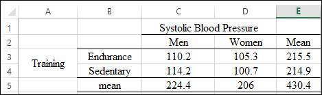
Graph: The problem compares two factors systolic blood pressure on y-axis with training level on x-axis. The factor systolic blood pressure is further classified for men and women and the other factor training level is classified to endurance trained and sedentary men and women. Thus, the table is created for the means of two factor as shown below;
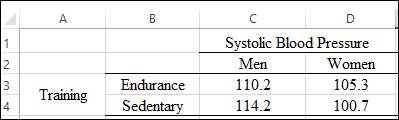
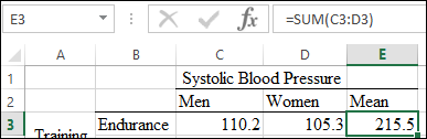
The marginal means for Endurance is calculated by using the
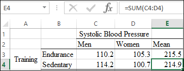
The marginal means for Sedentary is calculated by using the function
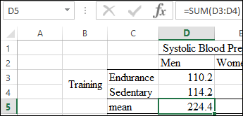
The marginal means for Systolic blood pressure for men is calculated by using the function
The marginal means for Systolic blood pressure for women is calculated by using the function
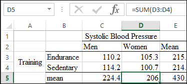
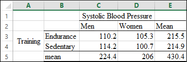
The table is obtained as:
The interaction plot is drawn by following these steps:
Step 1: Open Excel sheet and write the data value. The screenshot is shown below:
Step 2: INSERT>Recommended Charts>All Charts>Line Chart. The screenshot is shown below:
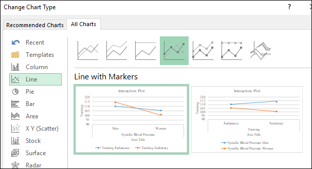
The interaction plot is obtained as shown below:
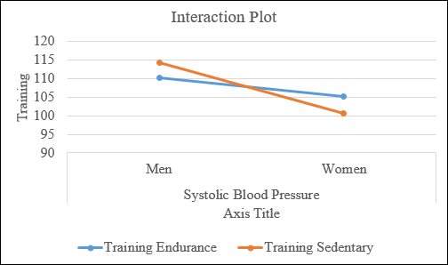
Interpretation: From the chart above, the two lines are not parallel, hence, there is an interaction present between two factors. There is a main effect of training level, training sedentary takes much lower value for women when compared to training endurance for women.
(b)
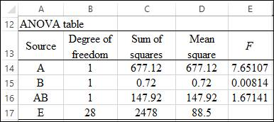
To find: The ANOVA table.
(b)
Answer to Problem 18E
Solution: The ANOVA table is obtained as:
Explanation of Solution
Given: The following values of the Sum of Squares is provided,
where A is the sex effect and B is the training level.
Calculation: The ANOVA table is obtained by following these steps:
Step 1: The degree of freedom for “A” is obtained as follows:
The degree of freedom for “B” is obtained as follows;
The degree of freedom for “AB” is obtained as follows:
The degree of freedom for “E” is obtained as follows:
Step 2: The
The mean squares for “B” is obtained as follows:
The mean squares for “AB” is obtained as follows:
The mean squares for “E” is obtained as follows:
Step 3: The F-value for “A” is obtained as follows:
The F-value for “B” is obtained as follows:
The F-value for “AB” is obtained as follows:
To test the hypothesis for the obtained F-values, the F-critical value is obtained through the F-distribution table as
Interpretation: The comparisons of F-values with F-critical are as follows:
The value of FA is greater than F-critical; hence, the null hypothesis can be rejected significantly, which states that there is a main effect of training level. While the other factor systolic blood pressure and the interaction of these two factors have F-value less than F-critical, which means that they do not show the significant difference in means.
(c)
The benefit of considering pretest measurement.
(c)
Answer to Problem 18E
Solution: It increases the power of the test statistic.
Explanation of Solution
Want to see more full solutions like this?
Chapter 13 Solutions
LaunchPad for Moore's Introduction to the Practice of Statistics (12 month access)


- Please could you check my answersarrow_forwardLet Y₁, Y2,, Yy be random variables from an Exponential distribution with unknown mean 0. Let Ô be the maximum likelihood estimates for 0. The probability density function of y; is given by P(Yi; 0) = 0, yi≥ 0. The maximum likelihood estimate is given as follows: Select one: = n Σ19 1 Σ19 n-1 Σ19: n² Σ1arrow_forwardPlease could you help me answer parts d and e. Thanksarrow_forward
- When fitting the model E[Y] = Bo+B1x1,i + B2x2; to a set of n = 25 observations, the following results were obtained using the general linear model notation: and 25 219 10232 551 XTX = 219 10232 3055 133899 133899 6725688, XTY 7361 337051 (XX)-- 0.1132 -0.0044 -0.00008 -0.0044 0.0027 -0.00004 -0.00008 -0.00004 0.00000129, Construct a multiple linear regression model Yin terms of the explanatory variables 1,i, x2,i- a) What is the value of the least squares estimate of the regression coefficient for 1,+? Give your answer correct to 3 decimal places. B1 b) Given that SSR = 5550, and SST=5784. Calculate the value of the MSg correct to 2 decimal places. c) What is the F statistics for this model correct to 2 decimal places?arrow_forwardCalculate the sample mean and sample variance for the following frequency distribution of heart rates for a sample of American adults. If necessary, round to one more decimal place than the largest number of decimal places given in the data. Heart Rates in Beats per Minute Class Frequency 51-58 5 59-66 8 67-74 9 75-82 7 83-90 8arrow_forwardcan someone solvearrow_forward
- QUAT6221wA1 Accessibility Mode Immersiv Q.1.2 Match the definition in column X with the correct term in column Y. Two marks will be awarded for each correct answer. (20) COLUMN X Q.1.2.1 COLUMN Y Condenses sample data into a few summary A. Statistics measures Q.1.2.2 The collection of all possible observations that exist for the random variable under study. B. Descriptive statistics Q.1.2.3 Describes a characteristic of a sample. C. Ordinal-scaled data Q.1.2.4 The actual values or outcomes are recorded on a random variable. D. Inferential statistics 0.1.2.5 Categorical data, where the categories have an implied ranking. E. Data Q.1.2.6 A set of mathematically based tools & techniques that transform raw data into F. Statistical modelling information to support effective decision- making. 45 Q Search 28 # 00 8 LO 1 f F10 Prise 11+arrow_forwardStudents - Term 1 - Def X W QUAT6221wA1.docx X C Chat - Learn with Chegg | Cheg X | + w:/r/sites/TertiaryStudents/_layouts/15/Doc.aspx?sourcedoc=%7B2759DFAB-EA5E-4526-9991-9087A973B894% QUAT6221wA1 Accessibility Mode பg Immer The following table indicates the unit prices (in Rands) and quantities of three consumer products to be held in a supermarket warehouse in Lenasia over the time period from April to July 2025. APRIL 2025 JULY 2025 PRODUCT Unit Price (po) Quantity (q0)) Unit Price (p₁) Quantity (q1) Mineral Water R23.70 403 R25.70 423 H&S Shampoo R77.00 922 R79.40 899 Toilet Paper R106.50 725 R104.70 730 The Independent Institute of Education (Pty) Ltd 2025 Q Search L W f Page 7 of 9arrow_forwardCOM WIth Chegg Cheg x + w:/r/sites/TertiaryStudents/_layouts/15/Doc.aspx?sourcedoc=%7B2759DFAB-EA5E-4526-9991-9087A973B894%. QUAT6221wA1 Accessibility Mode Immersi The following table indicates the unit prices (in Rands) and quantities of three meals sold every year by a small restaurant over the years 2023 and 2025. 2023 2025 MEAL Unit Price (po) Quantity (q0)) Unit Price (P₁) Quantity (q₁) Lasagne R125 1055 R145 1125 Pizza R110 2115 R130 2195 Pasta R95 1950 R120 2250 Q.2.1 Using 2023 as the base year, compute the individual price relatives in 2025 for (10) lasagne and pasta. Interpret each of your answers. 0.2.2 Using 2023 as the base year, compute the Laspeyres price index for all of the meals (8) for 2025. Interpret your answer. Q.2.3 Using 2023 as the base year, compute the Paasche price index for all of the meals (7) for 2025. Interpret your answer. Q Search L O W Larrow_forward
- QUAI6221wA1.docx X + int.com/:w:/r/sites/TertiaryStudents/_layouts/15/Doc.aspx?sourcedoc=%7B2759DFAB-EA5E-4526-9991-9087A973B894%7 26 QUAT6221wA1 Q.1.1.8 One advantage of primary data is that: (1) It is low quality (2) It is irrelevant to the purpose at hand (3) It is time-consuming to collect (4) None of the other options Accessibility Mode Immersive R Q.1.1.9 A sample of fifteen apples is selected from an orchard. We would refer to one of these apples as: (2) ھا (1) A parameter (2) A descriptive statistic (3) A statistical model A sampling unit Q.1.1.10 Categorical data, where the categories do not have implied ranking, is referred to as: (2) Search D (2) 1+ PrtSc Insert Delete F8 F10 F11 F12 Backspace 10 ENG USarrow_forwardepoint.com/:w:/r/sites/TertiaryStudents/_layouts/15/Doc.aspx?sourcedoc=%7B2759DFAB-EA5E-4526-9991-9087A 23;24; 25 R QUAT6221WA1 Accessibility Mode DE 2025 Q.1.1.4 Data obtained from outside an organisation is referred to as: (2) 45 (1) Outside data (2) External data (3) Primary data (4) Secondary data Q.1.1.5 Amongst other disadvantages, which type of data may not be problem-specific and/or may be out of date? W (2) E (1) Ordinal scaled data (2) Ratio scaled data (3) Quantitative, continuous data (4) None of the other options Search F8 F10 PrtSc Insert F11 F12 0 + /1 Backspaarrow_forward/r/sites/TertiaryStudents/_layouts/15/Doc.aspx?sourcedoc=%7B2759DFAB-EA5E-4526-9991-9087A973B894%7D&file=Qu Q.1.1.14 QUAT6221wA1 Accessibility Mode Immersive Reader You are the CFO of a company listed on the Johannesburg Stock Exchange. The annual financial statements published by your company would be viewed by yourself as: (1) External data (2) Internal data (3) Nominal data (4) Secondary data Q.1.1.15 Data relevancy refers to the fact that data selected for analysis must be: (2) Q Search (1) Checked for errors and outliers (2) Obtained online (3) Problem specific (4) Obtained using algorithms U E (2) 100% 高 W ENG A US F10 点 F11 社 F12 PrtSc 11 + Insert Delete Backspacearrow_forward
 MATLAB: An Introduction with ApplicationsStatisticsISBN:9781119256830Author:Amos GilatPublisher:John Wiley & Sons Inc
 Probability and Statistics for Engineering and th...StatisticsISBN:9781305251809Author:Jay L. DevorePublisher:Cengage Learning
 Statistics for The Behavioral Sciences (MindTap C...StatisticsISBN:9781305504912Author:Frederick J Gravetter, Larry B. WallnauPublisher:Cengage Learning
 Elementary Statistics: Picturing the World (7th E...StatisticsISBN:9780134683416Author:Ron Larson, Betsy FarberPublisher:PEARSON
 The Basic Practice of StatisticsStatisticsISBN:9781319042578Author:David S. Moore, William I. Notz, Michael A. FlignerPublisher:W. H. Freeman
 Introduction to the Practice of StatisticsStatisticsISBN:9781319013387Author:David S. Moore, George P. McCabe, Bruce A. CraigPublisher:W. H. Freeman