
Videos
(a)
To graph: The interaction plot displaying systolic blood pressure on the y-axis and training level on the x-axis.
(a)
Explanation of Solution
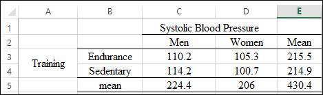
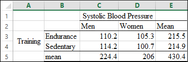
Graph: The problem compares two factors systolic blood pressure on y-axis with training level on x-axis. The factor systolic blood pressure is further classified for men and women and the other factor training level is classified to endurance trained and sedentary men and women. Thus, the table is created for the means of two factor as shown below;
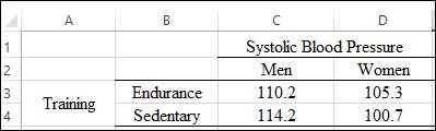
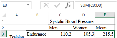
The marginal means for Endurance is calculated by using the
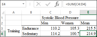
The marginal means for Sedentary is calculated by using the function
The marginal means for Systolic blood pressure for men is calculated by using the function
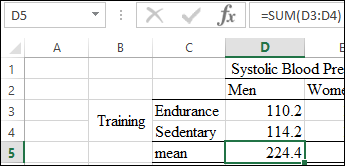
The marginal means for Systolic blood pressure for women is calculated by using the function
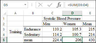
The table is obtained as:
The interaction plot is drawn by following these steps:
Step 1: Open Excel sheet and write the data value. The screenshot is shown below:
Step 2: INSERT>Recommended Charts>All Charts>Line Chart. The screenshot is shown below:
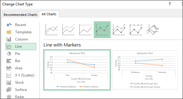
The interaction plot is obtained as shown below:
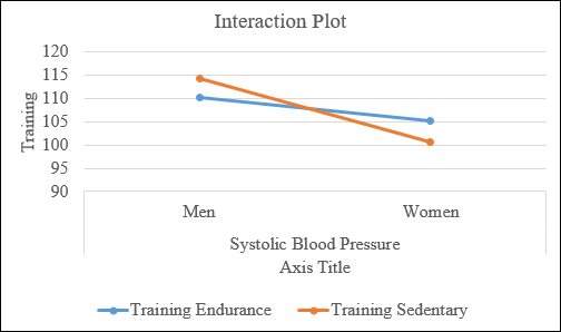
Interpretation: From the chart above, the two lines are not parallel, hence, there is an interaction present between two factors. There is a main effect of training level, training sedentary takes much lower value for women when compared to training endurance for women.
(b)
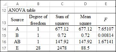
To find: The ANOVA table.
(b)
Answer to Problem 18E
Solution: The ANOVA table is obtained as:
Explanation of Solution
Given: The following values of the Sum of Squares is provided,
where A is the sex effect and B is the training level.
Calculation: The ANOVA table is obtained by following these steps:
Step 1: The degree of freedom for “A” is obtained as follows:
The degree of freedom for “B” is obtained as follows;
The degree of freedom for “AB” is obtained as follows:
The degree of freedom for “E” is obtained as follows:
Step 2: The
The mean squares for “B” is obtained as follows:
The mean squares for “AB” is obtained as follows:
The mean squares for “E” is obtained as follows:
Step 3: The F-value for “A” is obtained as follows:
The F-value for “B” is obtained as follows:
The F-value for “AB” is obtained as follows:
To test the hypothesis for the obtained F-values, the F-critical value is obtained through the F-distribution table as
Interpretation: The comparisons of F-values with F-critical are as follows:
The value of FA is greater than F-critical; hence, the null hypothesis can be rejected significantly, which states that there is a main effect of training level. While the other factor systolic blood pressure and the interaction of these two factors have F-value less than F-critical, which means that they do not show the significant difference in means.
(c)
The benefit of considering pretest measurement.
(c)
Answer to Problem 18E
Solution: It increases the power of the test statistic.
Explanation of Solution
Want to see more full solutions like this?
Chapter 13 Solutions
EBK INTRODUCTION TO THE PRACTICE OF STA


- A company found that the daily sales revenue of its flagship product follows a normal distribution with a mean of $4500 and a standard deviation of $450. The company defines a "high-sales day" that is, any day with sales exceeding $4800. please provide a step by step on how to get the answers in excel Q: What percentage of days can the company expect to have "high-sales days" or sales greater than $4800? Q: What is the sales revenue threshold for the bottom 10% of days? (please note that 10% refers to the probability/area under bell curve towards the lower tail of bell curve) Provide answers in the yellow cellsarrow_forwardFind the critical value for a left-tailed test using the F distribution with a 0.025, degrees of freedom in the numerator=12, and degrees of freedom in the denominator = 50. A portion of the table of critical values of the F-distribution is provided. Click the icon to view the partial table of critical values of the F-distribution. What is the critical value? (Round to two decimal places as needed.)arrow_forwardA retail store manager claims that the average daily sales of the store are $1,500. You aim to test whether the actual average daily sales differ significantly from this claimed value. You can provide your answer by inserting a text box and the answer must include: Null hypothesis, Alternative hypothesis, Show answer (output table/summary table), and Conclusion based on the P value. Showing the calculation is a must. If calculation is missing,so please provide a step by step on the answers Numerical answers in the yellow cellsarrow_forward
 MATLAB: An Introduction with ApplicationsStatisticsISBN:9781119256830Author:Amos GilatPublisher:John Wiley & Sons Inc
 Probability and Statistics for Engineering and th...StatisticsISBN:9781305251809Author:Jay L. DevorePublisher:Cengage Learning
 Statistics for The Behavioral Sciences (MindTap C...StatisticsISBN:9781305504912Author:Frederick J Gravetter, Larry B. WallnauPublisher:Cengage Learning
 Elementary Statistics: Picturing the World (7th E...StatisticsISBN:9780134683416Author:Ron Larson, Betsy FarberPublisher:PEARSON
 The Basic Practice of StatisticsStatisticsISBN:9781319042578Author:David S. Moore, William I. Notz, Michael A. FlignerPublisher:W. H. Freeman
 Introduction to the Practice of StatisticsStatisticsISBN:9781319013387Author:David S. Moore, George P. McCabe, Bruce A. CraigPublisher:W. H. Freeman