
(a)
Mathematical expression of marginal revenue product of labor.
(a)
Explanation of Solution
To derive the mathematical expression of marginal revenue product of labor, it is necessary to derive the intercept and slope of the MRPL.
The general formula for calculating slope of the MRPL curve is given as follows:
Substitute the respective values in Equation (1) to calculate the slope of MRPL.
Slope is
Substitute the slope in the general formula of equation to derive the expression of MRPL.
Substitute “MRPL” for “y” and “L’’ for “x”.
Mathematical expression of marginal revenue product of labor is
Marginal revenue product of labor: Marginal revenue product of labor is the change in the firm’s revenue as a result of employing an extra unit of labor.
(b)
Mathematical expression of supply of labor in the lemongrass industry.
(b)
Explanation of Solution
Substitute the respective values in Equation (1) to calculate the slope of supply curve.
Slope is 0.25.
Substitute the slope in the general formula of equation to derive the expression of supply curve.
Substitute “W” for “y” and “L’’ for “x”.
Mathematical expression of supply of labor is
(c)
Number workers hired and wage rate paid.
(c)
Explanation of Solution
The competitive outcome is characterized by equating the wage rate and the marginal revenue product of labor. Symbolically, it is shown below:
The value of “W” and “MRPL” is already calculated in part (a) and in part (b), respectively.
The number of laborers hired is 56 units.
Substitute the quantity of laborers hired in the supply curve of labor (Equation (3)).
Wage rate paid is $14.
(d)
Mathematical expression of marginal expenditure curve and draw the graph of the marginal expenditure curve.
(d)
Explanation of Solution
As per the rule of marginal expenditure, that is, marginal expenditure curve has twice the slope of the labor supply curve. The labor supply curve is
Marginal expenditure curve function is
Graphical illustration of marginal expenditure curve is depicted in the Figure below:
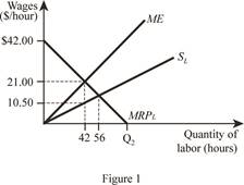
In Figure 1, the vertical axis measures wage rate, and horizontal axis measures quantity of labor. The downward sloping curve is the marginal revenue product of labor. The upward sloping curve SL is the supply curve of labor, and ME is the marginal expenditure curve of labor. The slope of marginal expenditure curve is twice the slope of supply curve of labor.
(e)
Units of labor will a monopsolistic lemongrass producer hire and wage rate paid.
(e)
Explanation of Solution
The monopsolistic outcome is characterized by equating the marginal revenue product of labor and marginal expenditure. Symbolically, it is shown below:
The values of “MRPL” and “ME” are already calculated in part (a) and part (c), respectively.
Units of labor will a monopsolistic lemongrass producer hire (Monopsony quantity) is 42 units.
Substitute the quantity of labor a monopsolistic producer hires in the supply curve of labor (Equation (3)).
Wage rate (Monopsony wage) paid is $10.5.
(f)
Fall in employment.
(f)
Explanation of Solution
The labor market goes from competitive on the buyer’s side to monopsonistic side, that result in decrease the employment. That is, at competitive market, the unit of laborers hired is 56, but in monopsonistic market, the unit of laborers hired is 42. Thus, the quantity of labor hired is reduced by 14 units
(g)
(g)
Explanation of Solution
Deadweight loss can be calculated as follows:
Thus, deadweight loss is $73.50.
The graphical illustration of deadweight loss is depicted below in Figure 2.
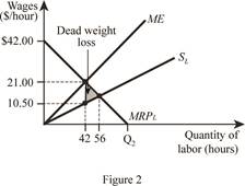
In Figure 2, the vertical axis measures wage rate, and horizontal axis measures quantity of labor. The downward sloping curve is the marginal revenue product of labor. The upward sloping curve SL is the supply curve of labor, and ME is the marginal expenditure curve of labor. The shaded area is the deadweight loss created in the society.
Want to see more full solutions like this?
Chapter 13 Solutions
Microeconomics

- agrody calming Inted 001 and me 2. A homeowner is concerned about the various air pollutants (e.g., benzene and methane) released in her house when she cooks with natural gas. She is considering replacing her gas oven and stove with an electric stove comprising an induction cooktop and convection oven. The new appliance costs $900 to purchase and install. Capping the old gas line costs an additional $150 (a one-time fee). The old line must be inspected for leaks each year after capping, at a cost of $35 for each inspection. a. If the homeowner plans to remain in the house for four more years and the discount rate is 4%, what is the minimum present value of the benefits that the homeowner would need to experience for this purchase to be justified based on its private net sub present value? b. While trying to understand how she might express the value of reduced exposure to indoor air pollutants in dollar terms, the homeowner consulted the EPA website and found estimates provided by…arrow_forwardAfter the ban is imposed, Joe’s firm switches to the more expensive biodegradable disposable cups. This increases the cost associated with each cup of coffee it produces. Which cost curve(s) will be impacted by the use of the more expensive biodegradable disposable cups? Why? Which cost curve(s) will not shift, and why not? Please use the table below to answer this question. For the second column (“Impacted? If so, how?”), please use one of the following three choices: No shift; Shifts up (i.e., increases: at nearly any given quantity, the cost goes up); or Shifts down (i.e., decreases: at nearly any given quantity, the cost goes down). $ Cost Curve Impacted? If so, how? Explanation of the Shift: Why or Why Not AFC No shift. Fix costs stay the same, regardless of quantity. Fixed cost is calculated as Fixed Cost/Quantity. Since fixed costs remain unchanged, AFC stays the same for each quantity. MC Shifts up. Since the biodegradable cups are more expensive, the…arrow_forwardStyrofoam is non-biodegradable and is not easily recyclable. Many cities and at least one state have enacted laws that ban the use of polystyrene containers. These locales understand that banning these containers will force many businesses to turn to other more expensive forms of packaging and cups, but argue the ban is environmentally important. Shane owns a firm with a conventional production function resulting in U-shaped ATC, AVC, and MC curves. Shane's business sells takeout food and drinks that are currently packaged in styrofoam containers and cups. Graph the short-run AFC0, AVC0, ATC0, and MC0 curves for Shane's firm before the ban on using styrofoam containers.arrow_forward
- PART II: Multipart Problems wood or solem of triflussd aidi 1. Assume that a society has a polluting industry comprising two firms, where the industry-level marginal abatement cost curve is given by: MAC = 24 - ()E and the marginal damage function is given by: MDF = 2E. What is the efficient level of emissions? b. What constant per-unit emissions tax could achieve the efficient emissions level? points) c. What is the net benefit to society of moving from the unregulated emissions level to the efficient level? In response to industry complaints about the costs of the tax, a cap-and-trade program is proposed. The marginal abatement cost curves for the two firms are given by: MAC=24-E and MAC2 = 24-2E2. d. How could a cap-and-trade program that achieves the same level of emissions as the tax be designed to reduce the costs of regulation to the two firms?arrow_forwardOnly #4 please, Use a graph please if needed to help provearrow_forwarda-carrow_forward
- For these questions, you must state "true," "false," or "uncertain" and argue your case (roughly 3 to 5 sentences). When appropriate, the use of graphs will make for stronger answers. Credit will depend entirely on the quality of your explanation. 1. If the industry facing regulation for its pollutant emissions has a lot of political capital, direct regulatory intervention will be more viable than an emissions tax to address this market failure. 2. A stated-preference method will provide a measure of the value of Komodo dragons that is more accurate than the value estimated through application of the travel cost model to visitation data for Komodo National Park in Indonesia. 3. A correlation between community demographics and the present location of polluting facilities is sufficient to claim a violation of distributive justice. olsvrc Q 4. When the damages from pollution are uncertain, a price-based mechanism is best equipped to manage the costs of the regulator's imperfect…arrow_forwardFor environmental economics, question number 2 only please-- thank you!arrow_forwardFor these questions, you must state "true," "false," or "uncertain" and argue your case (roughly 3 to 5 sentences). When appropriate, the use of graphs will make for stronger answers. Credit will depend entirely on the quality of your explanation. 1. If the industry facing regulation for its pollutant emissions has a lot of political capital, direct regulatory intervention will be more viable than an emissions tax to address this market failure. cullog iba linevoz ve bubivorearrow_forward

 Principles of Economics (12th Edition)EconomicsISBN:9780134078779Author:Karl E. Case, Ray C. Fair, Sharon E. OsterPublisher:PEARSON
 Engineering Economy (17th Edition)EconomicsISBN:9780134870069Author:William G. Sullivan, Elin M. Wicks, C. Patrick KoellingPublisher:PEARSON
 Principles of Economics (MindTap Course List)EconomicsISBN:9781305585126Author:N. Gregory MankiwPublisher:Cengage Learning
 Managerial Economics: A Problem Solving ApproachEconomicsISBN:9781337106665Author:Luke M. Froeb, Brian T. McCann, Michael R. Ward, Mike ShorPublisher:Cengage Learning
 Managerial Economics & Business Strategy (Mcgraw-...EconomicsISBN:9781259290619Author:Michael Baye, Jeff PrincePublisher:McGraw-Hill Education