
(a)
Mathematical expression of marginal revenue product of labor.
(a)
Explanation of Solution
To derive the mathematical expression of marginal revenue product of labor, it is necessary to derive the intercept and slope of the MRPL.
The general formula for calculating slope of the MRPL curve is given as follows:
Substitute the respective values in Equation (1) to calculate the slope of MRPL.
Slope is
Substitute the slope in the general formula of equation to derive the expression of MRPL.
Substitute “MRPL” for “y” and “L’’ for “x”.
Mathematical expression of marginal revenue product of labor is
Marginal revenue product of labor: Marginal revenue product of labor is the change in the firm’s revenue as a result of employing an extra unit of labor.
(b)
Mathematical expression of supply of labor in the lemongrass industry.
(b)
Explanation of Solution
Substitute the respective values in Equation (1) to calculate the slope of supply curve.
Slope is 0.25.
Substitute the slope in the general formula of equation to derive the expression of supply curve.
Substitute “W” for “y” and “L’’ for “x”.
Mathematical expression of supply of labor is
(c)
Number workers hired and wage rate paid.
(c)
Explanation of Solution
The competitive outcome is characterized by equating the wage rate and the marginal revenue product of labor. Symbolically, it is shown below:
The value of “W” and “MRPL” is already calculated in part (a) and in part (b), respectively.
The number of laborers hired is 56 units.
Substitute the quantity of laborers hired in the supply curve of labor (Equation (3)).
Wage rate paid is $14.
(d)
Mathematical expression of marginal expenditure curve and draw the graph of the marginal expenditure curve.
(d)
Explanation of Solution
As per the rule of marginal expenditure, that is, marginal expenditure curve has twice the slope of the labor supply curve. The labor supply curve is
Marginal expenditure curve function is
Graphical illustration of marginal expenditure curve is depicted in the Figure below:
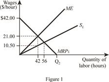
In Figure 1, the vertical axis measures wage rate, and horizontal axis measures quantity of labor. The downward sloping curve is the marginal revenue product of labor. The upward sloping curve SL is the supply curve of labor, and ME is the marginal expenditure curve of labor. The slope of marginal expenditure curve is twice the slope of supply curve of labor.
(e)
Units of labor will a monopsolistic lemongrass producer hire and wage rate paid.
(e)
Explanation of Solution
The monopsolistic outcome is characterized by equating the marginal revenue product of labor and marginal expenditure. Symbolically, it is shown below:
The values of “MRPL” and “ME” are already calculated in part (a) and part (c), respectively.
Units of labor will a monopsolistic lemongrass producer hire (Monopsony quantity) is 42 units.
Substitute the quantity of labor a monopsolistic producer hires in the supply curve of labor (Equation (3)).
Wage rate (Monopsony wage) paid is $10.5.
(f)
Fall in employment.
(f)
Explanation of Solution
The labor market goes from competitive on the buyer’s side to monopsonistic side, that result in decrease the employment. That is, at competitive market, the unit of laborers hired is 56, but in monopsonistic market, the unit of laborers hired is 42. Thus, the quantity of labor hired is reduced by 14 units
(g)
(g)
Explanation of Solution
Deadweight loss can be calculated as follows:
Thus, deadweight loss is $73.50.
The graphical illustration of deadweight loss is depicted below in Figure 2.
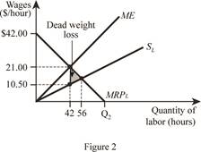
In Figure 2, the vertical axis measures wage rate, and horizontal axis measures quantity of labor. The downward sloping curve is the marginal revenue product of labor. The upward sloping curve SL is the supply curve of labor, and ME is the marginal expenditure curve of labor. The shaded area is the deadweight loss created in the society.
Want to see more full solutions like this?
Chapter 13 Solutions
EBK MICROECONOMICS

- You are the manager of a large automobile dealership who wants to learn more about the effective- ness of various discounts offered to customers over the past 14 months. Following are the average negotiated prices for each month and the quantities sold of a basic model (adjusted for various options) over this period of time. 1. Graph this information on a scatter plot. Estimate the demand equation. What do the regression results indicate about the desirability of discounting the price? Explain. Month Price Quantity Jan. 12,500 15 Feb. 12,200 17 Mar. 11,900 16 Apr. 12,000 18 May 11,800 20 June 12,500 18 July 11,700 22 Aug. 12,100 15 Sept. 11,400 22 Oct. 11,400 25 Nov. 11,200 24 Dec. 11,000 30 Jan. 10,800 25 Feb. 10,000 28 2. What other factors besides price might be included in this equation? Do you foresee any difficulty in obtaining these additional data or incorporating them in the regression analysis?arrow_forwardsimple steps on how it should look like on excelarrow_forwardConsider options on a stock that does not pay dividends.The stock price is $100 per share, and the risk-free interest rate is 10%.Thestock moves randomly with u=1.25and d=1/u Use Excel to calculate the premium of a10-year call with a strike of $100.arrow_forward
- Please solve this, no words or explanations.arrow_forward17. Given that C=$700+0.8Y, I=$300, G=$600, what is Y if Y=C+I+G?arrow_forwardUse the Feynman technique throughout. Assume that you’re explaining the answer to someone who doesn’t know the topic at all. Write explanation in paragraphs and if you use currency use USD currency: 10. What is the mechanism or process that allows the expenditure multiplier to “work” in theKeynesian Cross Model? Explain and show both mathematically and graphically. What isthe underpinning assumption for the process to transpire?arrow_forward
- Use the Feynman technique throughout. Assume that you’reexplaining the answer to someone who doesn’t know the topic at all. Write it all in paragraphs: 2. Give an overview of the equation of exchange (EoE) as used by Classical Theory. Now,carefully explain each variable in the EoE. What is meant by the “quantity theory of money”and how is it different from or the same as the equation of exchange?arrow_forwardZbsbwhjw8272:shbwhahwh Zbsbwhjw8272:shbwhahwh Zbsbwhjw8272:shbwhahwhZbsbwhjw8272:shbwhahwhZbsbwhjw8272:shbwhahwharrow_forwardUse the Feynman technique throughout. Assume that you’re explaining the answer to someone who doesn’t know the topic at all:arrow_forward

 Principles of Economics (12th Edition)EconomicsISBN:9780134078779Author:Karl E. Case, Ray C. Fair, Sharon E. OsterPublisher:PEARSON
 Engineering Economy (17th Edition)EconomicsISBN:9780134870069Author:William G. Sullivan, Elin M. Wicks, C. Patrick KoellingPublisher:PEARSON
 Principles of Economics (MindTap Course List)EconomicsISBN:9781305585126Author:N. Gregory MankiwPublisher:Cengage Learning
 Managerial Economics: A Problem Solving ApproachEconomicsISBN:9781337106665Author:Luke M. Froeb, Brian T. McCann, Michael R. Ward, Mike ShorPublisher:Cengage Learning
 Managerial Economics & Business Strategy (Mcgraw-...EconomicsISBN:9781259290619Author:Michael Baye, Jeff PrincePublisher:McGraw-Hill Education