Videos
Suppose that each firm in a competitive industry has the following costs:
Total cost: TC = 50 + ½ q2
Marginal cost: MC = q
where q is an individual firm’s quantity produced.
The market demand curve for this product is
Demand: QD = 120 − P
where P is the
a. What is each firm’s fixed cost? What is its variable cost? Give the equation for
b. Graph average-total-cost curve and the marginal-cost curve for q from 5 to 15. At what quantity is average-total-cost curve at its minimum? What is marginal cost and average total cost at that quantity?
c Give the equation for each firm’s supply curve.
d. Give the equation for the market supply curve for the short run in which the number of firms is fixed.
e. What is the
f. In this equilibrium, how much does each firm produce? Calculate each firm’s profit or loss. Is there incentive for firms to enter or exit?
g. In the long run with free entry and exit, what is the equilibrium price and quantity in this market?
h. In this long-run equilibrium, how much does each firm produce? How many firms are in the market?
Subpart (a):
Calculate average total cost.
Explanation of Solution
The total cost equation, marginal cost equation and demand equation are given below:
The fixed cost and variable cost of each firm are determined from Equation (1). Here, the fixed cost is a part of the total cost and will not change in response to a change in quantity. The variable cost is a part of the total cost and it changes in response to a change in quantity. So, the fixed cost is $50 and the variable cost is
Average total cost equation is represented below:
Or
Concept introduction:
Average total cost: The average total cost is the total cost per unit of the output produced by a firm.
Subpart (b):
Draw average total cost curve.
Explanation of Solution
Figure 1 represents the average total cost curve and marginal cost curve.
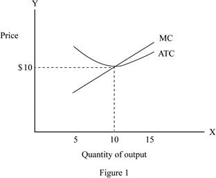
From the above figure, the x-axis shows the quantity of the output and the y-axis shows the price level.
From the graph, the average total cost is at its minimum, when they produce 10 units of output. The average total cost and marginal cost are at the quantity of 10 units of output.
Concept introduction:
Average total cost: The average total cost is the total cost per unit of the output produced by a firm.
Subpart (c):
Supply curve.
Explanation of Solution
In the perfect competition, the supply curve is even, as the marginal cost curve is beyond the intersecting point of the average total cost curve.
Supply curve for each firm is shown below:
Concept introduction:
Marginal cost curve: The marginal cost is the additional cost incurred on the additional production and its curve is U-shaped, which represents the combination of price level and quantity of output.
Subpart (d):
Quantity supply.
Explanation of Solution
In the short-run, there are currently 9 firms. So, the market supply curve is determined by using the following formula:
Hence, the short-run market supply curve is shown below:
Concept introduction:
Supply: Supply refers to the total value of the goods and services that are available for the purchase at a particular price in a given period of time.
Subpart (e):
Equilibrium price and quantity.
Explanation of Solution
The equilibrium quantity and price are determined by using the following formula:
Substitute the respective values in Equation (8) to calculate the equilibrium quantity and price.
Thus, the equilibrium price is $12.
Substitute the price of $12 in Equation (3) to calculate the equilibrium quantity.
Thus, the equilibrium quantity is 108 units.
Concept introduction:
Equilibrium price: It is the price at which the quantity demanded of a good or service is equal to the quantity supplied.
Equilibrium: It is the market price and quantity determined by equating the supply to the demand. At this equilibrium point, the supply will be equal to the demand and there will be no excess demand or supply in the economy. Thus, the economy will be at equilibrium.
Subpart (f):
Calculate profit.
Explanation of Solution
In the short-run equilibrium, each firm produces 12 units
Profit can be calculated by using the following formula:
Substitute the respective values in Equation (9) to calculate the profit.
Thus, the profit is $22.
Since the firms have positive value in making profit, there will be a benefit for the firm entering the market.
Concept introduction:
Profit: Profit refers to the excess revenue after subtracting the total cost from the total revenue.
Subpart (g):
Equilibrium quantity.
Explanation of Solution
In the long-run, the firm earns zero economic profit, so the price is equal to the minimum average total cost. Since the average total cost is $10, the equilibrium price is also be $10.
Equilibrium quantity can be determined by using Equation (3), when the equilibrium price is $10.
Thus, the long-run equilibrium quantity is 110.
Concept introduction:
Equilibrium: It is the market price and quantity determined by equating the supply to the demand. At this equilibrium point, the supply will be equal to the demand and there will be no excess demand or supply in the economy. Thus, the economy will be at equilibrium.
Subpart (h):
Number of firms in the long run.
Explanation of Solution
In the long-run, the firm produces 10 units of output. This is because in the long-run, the production price of the firm is equal to the minimum average total cost. The average total cost is 10 units. Also, there are 11 firms
Long run: Thelong run refers to the time, which changes the production variable to adjust to the market situation.
Want to see more full solutions like this?
Chapter 13 Solutions
EBK ESSENTIALS OF ECONOMICS


- If the US Federal Reserve increases interests on reserves, how will that change the original equilibrium shown in the graph? Euros par US alar 1.10 1.00 0.90- E 0.80- 0.70 0.60 0.50 0.40- 0.30 0.20 47 48 49 50 51 52 53 54 55 56 Quantity of US Dollars traded for Euros (trillions/day) It will increase the demand for Dollars and decrease the supply, so the exchange rate decreases, and the quantity traded increases. O It will decrease the demand for Dollars and increase the supply, so the exchange rate decreases and the impact on the quantity traded is unknown. O It will increase the demand for Dollars and decrease the supply, so the exchange rate increases and the impact on the quantity traded is unknown O It will decrease the demand for Dollars and increase the supply, so the exchange rate decreases, and the quantity traded increases. Question 22 5 ptsarrow_forward1. Based on the video, answer the following questions. • What are the 5 key characteristics that differentiate perfect competition from monopoly? Based on the video. • How does the number of sellers in a market influence the type of market structure? Based on the video. • In what ways does product differentiation play a role in monopolistic competition? Based on the video. • How do barriers to entry affect the level of competition in an oligopoly? Based on the video. • Why might firms in an oligopolistic market engage in non-price competition rather than price wars? Based on the video. Reference video: https://youtu.be/Qrr-IGR1kvE?si=h4q2F1JFNoCI36TVarrow_forward1. Answer the following questions based on the reference video below: • What are the 5 key characteristics that differentiate perfect competition from monopoly? • How does the number of sellers in a market influence the type of market structure? • In what ways does product differentiation play a role in monopolistic competition? • How do barriers to entry affect the level of competition in an oligopoly? • Why might firms in an oligopolistic market engage in non-price competition rather than price wars? Discuss. Reference video: https://youtu.be/Qrr-IGR1kvE?si=h4q2F1JFNoCI36TVarrow_forward
- Explain the importance of differential calculus within economics and business analysis. Provide three refernces with your answer. They can be from websites or a journals.arrow_forwardAnalyze the graph below, showing the Gross Federal Debt as a percentage of GDP for the United States (1939-2019). Which of the following is correct? FRED Gross Federal Debt as Percent of Gross Domestic Product Percent of GDP 120 110 100 60 50 40 90 30 1940 1950 1960 1970 Shaded areas indicate US recessions 1980 1990 2000 2010 1000 Sources: OMD, St. Louis Fed myfred/g/U In 2019, the Federal Government of the United States had an accumulated debt/GDP higher than 100%, meaning that the amount of debt accumulated over time is higher than the value of all goods and services produced in that year. The debt/GDP is always positive during this period, so the Federal Government of the United States incurred in budget deficits every year since 1939. From the mid-40s until the mid-70s, the debt/DGP was decreasing, meaning that the Federal Government of the United States was running a budget surplus every year during those three decades. During the second half of the 1970s, the Federal Government…arrow_forwardAn imaginary country estimates that their economy can be approximated by the AD/AS model below. How can this government act to move the equilibrium to potential GDP? LRAS Price Level P Y Real GDP E SRAS AD The AD/AS model shows that a contractionary fiscal policy is suitable, but the choice of increasing taxes, decreasing government expenditure or doing both simultaneously is mostly political The AD/AS model shows that increasing taxes is the best fiscal policy available. The AD/AS model shows that decreasing government expenditure is the best fiscal policy available. The AD/AS model shows that an expansionary fiscal policy capable of shifting the AD curve to the potential GDP level would decrease Real GDP but increase inflationary pressuresarrow_forward
- Question 1 Coursology Consider the four policies bellow. Classify them as either fiscal or monetary policy: I. The United States Government promoting tax cuts for small businesses to prevent a wave of bankruptcies during the COVID-19 pandemic II. The Congress approving a higher budget for the Affordable Health Care Act (also known as Obamacare) III. The Federal Reserve increasing the required reserves for commercial banks aiming to control the rise of inflation IV. President Joe Biden approving a new round of stimulus checks for households I. fiscal, II. fiscal, III. monetary, IV. fiscal I. fiscal, II. monetary, III. monetary, IV. monetary I. monetary, II. fiscal, III. fiscal, IV. fiscal I. monetary, II. monetary, III. fiscal, IV. monetaryarrow_forwardConsider the following supply and demand schedule of wooden tables.a. Draw the corresponding graphs for supply and demand.b. Using the data, obtain the corresponding supply and demand functions. c. Find the market-clearing price and quantity. Price (Thousand s USD Supply Demand 2 96 1104 196 1906 296 2708 396 35010 496 43012 596 51014 696 59016 796 67018 896 75020…arrow_forwardConsider a firm with the following production function Q=5000L-2L2.a. Find the maximum production level.b. How many units of labour are needed at that point. c. Obtain the function of marginal product of labour (MRL) d. Graph the production function and the MRL.arrow_forward
- Exercise 4A firm has the following total cost function TC=100q-5q2+0.5q3. Find the average cost function.arrow_forwardA firm has the following demand function P=200 − 2Q and the average costof AC= 100/Q + 3Q −20.a. Find the profit function. b. Estimate the marginal cost function. c. Obtain the production that maximizes the profit. d. Evaluate the average cost and the marginal cost at the maximising production level.arrow_forwardRubber: Initial investment: $159,000 Annual cost: $36,000 Annual revenue: $101,000 Salvage value: $12,000 Useful life: 10 years Using the cotermination assumptions, a study period of 6 years, and a MARR of 9%, what is the present worth of the rubber alternative? Assume that the rubber alternative's equipment has a market value of $18,000 at the end of Year 6.arrow_forward

 Economics (MindTap Course List)EconomicsISBN:9781337617383Author:Roger A. ArnoldPublisher:Cengage Learning
 Managerial Economics: A Problem Solving ApproachEconomicsISBN:9781337106665Author:Luke M. Froeb, Brian T. McCann, Michael R. Ward, Mike ShorPublisher:Cengage Learning
 Microeconomics: Private and Public Choice (MindTa...EconomicsISBN:9781305506893Author:James D. Gwartney, Richard L. Stroup, Russell S. Sobel, David A. MacphersonPublisher:Cengage Learning
 Economics: Private and Public Choice (MindTap Cou...EconomicsISBN:9781305506725Author:James D. Gwartney, Richard L. Stroup, Russell S. Sobel, David A. MacphersonPublisher:Cengage Learning