Concept Introduction
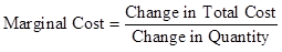
Marginal Cost: This refers to the change in the cost which is incurred when an additional unit of any good or service is produced. It shall be calculated as follows:
Shut-down
Explanation of Solution
a. Graph to show Bob’s marginal cost curve.
The below table shows the calculation of marginal cost:
| Quantity Produced(A) | Change in Quantity(B) | Fixed Cost($)(C) | Variable Cost($)(D) | Total Cost($)(E) | Change in Total Cost($)(F) | Marginal Cost($) |
| 0 | - | 50,000 | 0 | 50,000 | - | - |
| 1,000 | 1,000 | 50,000 | 5,000 | 55,000 | 5,000 | 5 |
| 2,000 | 1,000 | 50,000 | 8,000 | 58,000 | 3,000 | 3 |
| 3,000 | 1,000 | 50,000 | 9,000 | 59,000 | 1,000 | 1 |
| 4,000 | 1,000 | 50,000 | 14,000 | 64,000 | 5,000 | 5 |
| 5,000 | 1,000 | 50,000 | 20,000 | 70,000 | 6,000 | 6 |
| 6,000 | 1,000 | 50,000 | 33,000 | 83,000 | 13,000 | 13 |
| 7,000 | 1,000 | 50,000 | 49,000 | 99,000 | 16,000 | 16 |
| 8,000 | 1,000 | 50,000 | 72,000 | 122,000 | 23,000 | 23 |
| 9,000 | 1,000 | 50,000 | 99,000 | 149,000 | 27,000 | 27 |
| 10,000 | 1,000 | 50,000 | 150,000 | 200,000 | 51,000 | 51 |
As per the marginal cost calculated in the above table, below is the graph that shows Bob’s marginal cost curve:
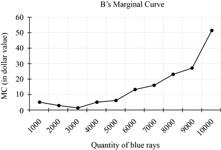
Fig 1
Conclusion:
Thus, the above graph shows the marginal curve drawn from the marginal costs calculated.
b. Range of price over which Mr. Bob will produce no units.
The below table shows the calculation of average variable cost:
| Quantity Produced(A) | Variable Cost($)(B) | Average Variable Cost($) |
| 0 | 0 | 0 |
| 1,000 | 5,000 | 5 |
| 2,000 | 8,000 | 4 |
| 3,000 | 9,000 | 3 |
| 4,000 | 14,000 | 3.5 |
| 5,000 | 20,000 | 4 |
| 6,000 | 33,000 | 5.5 |
| 7,000 | 49,000 | 7 |
| 8,000 | 72,000 | 7 |
| 9,000 | 99,000 | 11 |
| 10,000 | 150,000 | 15 |
Shut-down price is the level when the price is equal to the lowest average variable cost. Thus, as per the above table, the shut-down price is $3.
Mr. Bob will not produce any quantity when the price of a product falls below the shut-down price, which is $3. Hence, the range of price over which there will be no production is $0 to $3.
Conclusion:
Thus, the range of prices where there will be no production is $0 to $3.
c. Graph to show Mr. Bob’s individual supply curve.
The below table shows the marginal cost and average variable cost of Mr. Bob:
| Quantity Produced | Marginal Cost($) | Average Variable Cost($) |
| 0 | - | 0 |
| 1,000 | 5 | 5 |
| 2,000 | 3 | 4 |
| 3,000 | 1 | 3 |
| 4,000 | 5 | 3.5 |
| 5,000 | 6 | 4 |
| 6,000 | 13 | 5.5 |
| 7,000 | 16 | 7 |
| 8,000 | 23 | 7 |
| 9,000 | 27 | 11 |
| 10,000 | 51 | 15 |
As per the marginal cost and average variable cost in the above table, below is the graph that shows Bob’s individual supply curve:
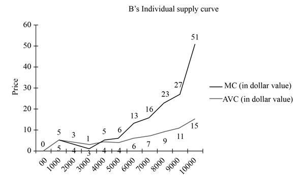
Fig 2
- The above graph shows that Mr. Bob will continue the production only if the price is above $3 which is the shut-down price.
- Hence, the production level at prices below the shut-down price of $3 is nil.
Conclusion:
Thus, the graph is shown for Mr. Bob’s individual supply curve.
Want to see more full solutions like this?

- simple steps on how it should look like on excelarrow_forwardConsider options on a stock that does not pay dividends.The stock price is $100 per share, and the risk-free interest rate is 10%.Thestock moves randomly with u=1.25and d=1/u Use Excel to calculate the premium of a10-year call with a strike of $100.arrow_forwardCompute the Fourier sine and cosine transforms of f(x) = e.arrow_forward
- 17. Given that C=$700+0.8Y, I=$300, G=$600, what is Y if Y=C+I+G?arrow_forwardUse the Feynman technique throughout. Assume that you’re explaining the answer to someone who doesn’t know the topic at all. Write explanation in paragraphs and if you use currency use USD currency: 10. What is the mechanism or process that allows the expenditure multiplier to “work” in theKeynesian Cross Model? Explain and show both mathematically and graphically. What isthe underpinning assumption for the process to transpire?arrow_forwardUse the Feynman technique throughout. Assume that you’reexplaining the answer to someone who doesn’t know the topic at all. Write it all in paragraphs: 2. Give an overview of the equation of exchange (EoE) as used by Classical Theory. Now,carefully explain each variable in the EoE. What is meant by the “quantity theory of money”and how is it different from or the same as the equation of exchange?arrow_forward
- Zbsbwhjw8272:shbwhahwh Zbsbwhjw8272:shbwhahwh Zbsbwhjw8272:shbwhahwhZbsbwhjw8272:shbwhahwhZbsbwhjw8272:shbwhahwharrow_forwardUse the Feynman technique throughout. Assume that you’re explaining the answer to someone who doesn’t know the topic at all:arrow_forwardUse the Feynman technique throughout. Assume that you’reexplaining the answer to someone who doesn’t know the topic at all: 4. Draw a Keynesian AD curve in P – Y space and list the shift factors that will shift theKeynesian AD curve upward and to the right. Draw a separate Classical AD curve in P – Yspace and list the shift factors that will shift the Classical AD curve upward and to the right.arrow_forward

 Principles of Economics (12th Edition)EconomicsISBN:9780134078779Author:Karl E. Case, Ray C. Fair, Sharon E. OsterPublisher:PEARSON
 Engineering Economy (17th Edition)EconomicsISBN:9780134870069Author:William G. Sullivan, Elin M. Wicks, C. Patrick KoellingPublisher:PEARSON
 Principles of Economics (MindTap Course List)EconomicsISBN:9781305585126Author:N. Gregory MankiwPublisher:Cengage Learning
 Managerial Economics: A Problem Solving ApproachEconomicsISBN:9781337106665Author:Luke M. Froeb, Brian T. McCann, Michael R. Ward, Mike ShorPublisher:Cengage Learning
 Managerial Economics & Business Strategy (Mcgraw-...EconomicsISBN:9781259290619Author:Michael Baye, Jeff PrincePublisher:McGraw-Hill Education