
Concept explainers
Videos
a.
Find whether there is a difference in the variation in team salary among the people from Country A and National league teams.
a.
Answer to Problem 50DE
There is no difference in the variance in team salary among the people from Country A and National league teams.
Explanation of Solution
The null and alternative hypotheses are stated below:
Null hypothesis: There is no difference in the variance in team salary among Country A and National league teams.
Alternative hypothesis: There is difference in the variance in team salary among Country A and National league teams.
Step-by-step procedure to obtain the test statistic using Excel:
- In the first column, enter the salaries of Country A’s team.
- In the second column, enter the salaries of National team.
- Select the Data tab on the top menu.
- Select Data Analysis and Click on: F-Test, Two-sample for variances and then click on OK.
- In the dialog box, select Input
Range . - Click OK
Output obtained using Excel is represented as follows:
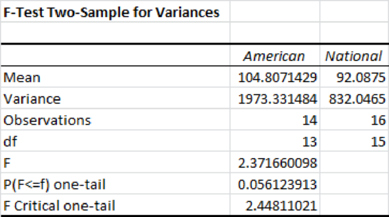
From the above output, the F- test statistic value is 2.37 and its p-value is 0.056.
Decision Rule:
If the p-value is less than the level of significance, reject the null hypothesis. Otherwise, fail to reject the null hypothesis.
Conclusion:
The significance level is 0.05. The p-value is 0.056 and it is greater than the significance level. The null hypothesis is rejected at the 0.05 significance level.
Thus, there is no difference in the variance in team salary among Country A and National league teams.
b.
Create a variable that classifies a team’s total attendance into three groups.
Find whether there is a difference in the
b.
Answer to Problem 50DE
There is no difference in the mean number of games won among the three groups.
Explanation of Solution
Let X represent the total attendance into three groups. Samples 1, 2, and 3 are “less than 2 (million)”, 2 up to 3, and 3 or more attendance of teams of three groups, respectively.
The following table gives the number of games won by the three groups of attendances.
| Sample 1 | Sample 2 | Sample 3 |
| 85 | 81 | 69 |
| 68 | 94 | 88 |
| 55 | 93 | 89 |
| 72 | 61 | 86 |
| 94 | 97 | 74 |
| 75 | 64 | 81 |
| 69 | 94 | |
| 83 | 88 | |
| 66 | 93 | |
| 95 | ||
| 79 | ||
| 76 | ||
| 73 | ||
| 98 |
The null and alternative hypotheses are as follows:
Null hypothesis: There is no difference in the mean number of games won among the three groups.
Alternative hypothesis: There is a difference in the mean number of games won among the three groups
Step-by-step procedure to obtain the test statistic using Excel:
- In Sample 1, enter the number of games won by the team, which is less than 2 million attendances.
- In Sample 2, enter the number of games won by the team of 2 up to 3 million attendances.
- In Sample 3, enter the number of games won by the team of 3 or more million attendances.
- Select the Data tab on the top menu.
- Select Data Analysis and Click on: ANOVA: Single factor and then click on OK.
- In the dialog box, select Input Range.
- Click OK
Output obtained using Excel is represented as follows:
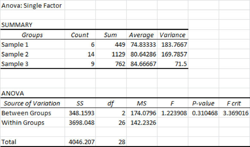
From the above output, the F test statistic value is 1.22 and the p-value is 0.31.
Conclusion:
The level of significance is 0.05. The p-value is greater than the significance level. Hence, one can fail to reject the null hypothesis at the 0.05 significance level. Thus, there is no difference in the mean number of games won among the three groups.
c.
Find whether there is a difference in the mean number of home runs hit per team using the variable defined in Part b.
c.
Answer to Problem 50DE
There is no difference in the mean number of home runs hit per team.
Explanation of Solution
The null and alternative hypotheses are stated below:
Null hypothesis: There is no difference in the mean number of home runs hit per team.
Alternative hypothesis: There is a difference in the mean number of home runs hit per team.
The following table gives the number of home runs per each team, which is defined in Part b.
| Sample 1 | Sample 2 | Sample 3 |
| 211 | 165 | 165 |
| 136 | 149 | 163 |
| 146 | 214 | 187 |
| 131 | 137 | 116 |
| 195 | 172 | 245 |
| 149 | 166 | 158 |
| 175 | 137 | 103 |
| 202 | 159 | |
| 131 | 200 | |
| 139 | ||
| 170 | ||
| 121 | ||
| 198 | ||
| 194 |
Step-by-step procedure to obtain the test statistic using Excel:
- In Sample 1, enter the number of home runs hit by the group of less than 2 million attendances.
- In Sample 2, enter the number of home runs hit by the group of 2 up to 3 million attendances.
- In Sample 3, enter the number of home runs hit by the group of 3 or more million attendances.
- Select the Data tab on the top menu.
- Select Data Analysis and Click on: ANOVA: Single factor and then click on OK.
- In the dialog box, select Input Range.
- Click OK
Output obtained using Excel is represented as follows:
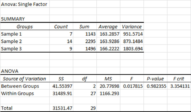
From the above output, the F test statistic value is 0.018 and the p-value is 0.9823.
Conclusion:
The level of significance is 0.05 and the p-value is greater than the significance level. Hence, one fails to reject the null hypothesis at the 0.05 significance level. Thus, there is no difference in the mean number of home runs hit per team.
d.
Find whether there is a difference in the mean salary of the three groups.
d.
Answer to Problem 50DE
The mean salaries are different for each group.
Explanation of Solution
The null and alternative hypotheses are stated below:
Null hypothesis: The mean salary of the three groups is equal.
Alternative hypothesis: At least one mean salary is different from other.
The following table provides the salary of each group that is defined in Part b.
| Sample 1 | Sample 2 | Sample 3 |
| 96.9 | 74.3 | 173.2 |
| 78.4 | 83.3 | 132.3 |
| 60.7 | 81.4 | 154.5 |
| 60.9 | 88.2 | 95.1 |
| 55.4 | 82.2 | 198 |
| 82 | 78.1 | 174.5 |
| 64.2 | 118.1 | 117.6 |
| 97.7 | 110.3 | |
| 94.1 | 120.5 | |
| 93.4 | ||
| 63.4 | ||
| 55.2 | ||
| 75.5 | ||
| 81.3 |
Step-by-step procedure to obtain the test statistic using Excel:
- In Sample 1, enter the salary of the group of less than 2 million attendances.
- In Sample 2, enter the salary of the group of 2 up to 3 million attendances.
- In Sample 3, enter the salary of the group of 3 or more million attendances.
- Select the Data tab on the top menu.
- Select Data Analysis and Click on: ANOVA: Single factor and then click on OK.
- In the dialog box, select Input Range.
- Click OK
Output obtained using Excel is represented as follows:
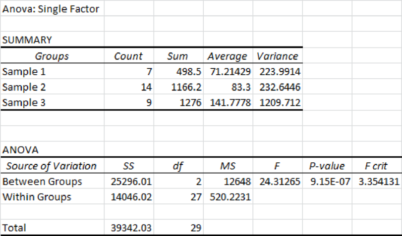
From the above output, the F test statistic value is 24.31 and the p-value is 0.
Conclusion:
The level of significance is 0.05 and the p-value is less than the significance level. Hence, one can reject the null hypothesis at the 0.05 significance level. Thus, the mean salaries are different for each group.
Want to see more full solutions like this?
Chapter 12 Solutions
Loose Leaf for Statistical Techniques in Business and Economics (Mcgraw-hill/Irwin Series in Operations and Decision Sciences)


- (a) What is a bimodal histogram? (b) Explain the difference between left-skewed, symmetric, and right-skewed histograms. (c) What is an outlierarrow_forward(a) Test the hypothesis. Consider the hypothesis test Ho = : against H₁o < 02. Suppose that the sample sizes aren₁ = 7 and n₂ = 13 and that $² = 22.4 and $22 = 28.2. Use α = 0.05. Ho is not ✓ rejected. 9-9 IV (b) Find a 95% confidence interval on of 102. Round your answer to two decimal places (e.g. 98.76).arrow_forwardLet us suppose we have some article reported on a study of potential sources of injury to equine veterinarians conducted at a university veterinary hospital. Forces on the hand were measured for several common activities that veterinarians engage in when examining or treating horses. We will consider the forces on the hands for two tasks, lifting and using ultrasound. Assume that both sample sizes are 6, the sample mean force for lifting was 6.2 pounds with standard deviation 1.5 pounds, and the sample mean force for using ultrasound was 6.4 pounds with standard deviation 0.3 pounds. Assume that the standard deviations are known. Suppose that you wanted to detect a true difference in mean force of 0.25 pounds on the hands for these two activities. Under the null hypothesis, 40 = 0. What level of type II error would you recommend here? Round your answer to four decimal places (e.g. 98.7654). Use a = 0.05. β = i What sample size would be required? Assume the sample sizes are to be equal.…arrow_forward
- = Consider the hypothesis test Ho: μ₁ = μ₂ against H₁ μ₁ μ2. Suppose that sample sizes are n₁ = 15 and n₂ = 15, that x1 = 4.7 and X2 = 7.8 and that s² = 4 and s² = 6.26. Assume that o and that the data are drawn from normal distributions. Use απ 0.05. (a) Test the hypothesis and find the P-value. (b) What is the power of the test in part (a) for a true difference in means of 3? (c) Assuming equal sample sizes, what sample size should be used to obtain ẞ = 0.05 if the true difference in means is - 2? Assume that α = 0.05. (a) The null hypothesis is 98.7654). rejected. The P-value is 0.0008 (b) The power is 0.94 . Round your answer to four decimal places (e.g. Round your answer to two decimal places (e.g. 98.76). (c) n₁ = n2 = 1 . Round your answer to the nearest integer.arrow_forwardConsider the hypothesis test Ho: = 622 against H₁: 6 > 62. Suppose that the sample sizes are n₁ = 20 and n₂ = 8, and that = 4.5; s=2.3. Use a = 0.01. (a) Test the hypothesis. Round your answers to two decimal places (e.g. 98.76). The test statistic is fo = i The critical value is f = Conclusion: i the null hypothesis at a = 0.01. (b) Construct the confidence interval on 02/022 which can be used to test the hypothesis: (Round your answer to two decimal places (e.g. 98.76).) iarrow_forward2011 listing by carmax of the ages and prices of various corollas in a ceratin regionarrow_forward
- س 11/ أ . اذا كانت 1 + x) = 2 x 3 + 2 x 2 + x) هي متعددة حدود محسوبة باستخدام طريقة الفروقات المنتهية (finite differences) من جدول البيانات التالي للدالة (f(x . احسب قيمة . ( 2 درجة ) xi k=0 k=1 k=2 k=3 0 3 1 2 2 2 3 αarrow_forward1. Differentiate between discrete and continuous random variables, providing examples for each type. 2. Consider a discrete random variable representing the number of patients visiting a clinic each day. The probabilities for the number of visits are as follows: 0 visits: P(0) = 0.2 1 visit: P(1) = 0.3 2 visits: P(2) = 0.5 Using this information, calculate the expected value (mean) of the number of patient visits per day. Show all your workings clearly. Rubric to follow Definition of Random variables ( clearly and accurately differentiate between discrete and continuous random variables with appropriate examples for each) Identification of discrete random variable (correctly identifies "number of patient visits" as a discrete random variable and explains reasoning clearly.) Calculation of probabilities (uses the probabilities correctly in the calculation, showing all steps clearly and logically) Expected value calculation (calculate the expected value (mean)…arrow_forwardif the b coloumn of a z table disappeared what would be used to determine b column probabilitiesarrow_forward
- Construct a model of population flow between metropolitan and nonmetropolitan areas of a given country, given that their respective populations in 2015 were 263 million and 45 million. The probabilities are given by the following matrix. (from) (to) metro nonmetro 0.99 0.02 metro 0.01 0.98 nonmetro Predict the population distributions of metropolitan and nonmetropolitan areas for the years 2016 through 2020 (in millions, to four decimal places). (Let x, through x5 represent the years 2016 through 2020, respectively.) x₁ = x2 X3 261.27 46.73 11 259.59 48.41 11 257.96 50.04 11 256.39 51.61 11 tarrow_forwardIf the average price of a new one family home is $246,300 with a standard deviation of $15,000 find the minimum and maximum prices of the houses that a contractor will build to satisfy 88% of the market valuearrow_forward21. ANALYSIS OF LAST DIGITS Heights of statistics students were obtained by the author as part of an experiment conducted for class. The last digits of those heights are listed below. Construct a frequency distribution with 10 classes. Based on the distribution, do the heights appear to be reported or actually measured? Does there appear to be a gap in the frequencies and, if so, how might that gap be explained? What do you know about the accuracy of the results? 3 4 555 0 0 0 0 0 0 0 0 0 1 1 23 3 5 5 5 5 5 5 5 5 5 5 5 5 6 6 8 8 8 9arrow_forward
 Big Ideas Math A Bridge To Success Algebra 1: Stu...AlgebraISBN:9781680331141Author:HOUGHTON MIFFLIN HARCOURTPublisher:Houghton Mifflin Harcourt
 Glencoe Algebra 1, Student Edition, 9780079039897...AlgebraISBN:9780079039897Author:CarterPublisher:McGraw Hill
 Holt Mcdougal Larson Pre-algebra: Student Edition...AlgebraISBN:9780547587776Author:HOLT MCDOUGALPublisher:HOLT MCDOUGAL