
Concept explainers
Videos
a.
Find whether there is a difference in the variation in team salary among the people from Country A and National league teams.
a.
Answer to Problem 50DE
There is no difference in the variance in team salary among the people from Country A and National league teams.
Explanation of Solution
The null and alternative hypotheses are stated below:
Null hypothesis: There is no difference in the variance in team salary among Country A and National league teams.
Alternative hypothesis: There is difference in the variance in team salary among Country A and National league teams.
Step-by-step procedure to obtain the test statistic using Excel:
- In the first column, enter the salaries of Country A’s team.
- In the second column, enter the salaries of National team.
- Select the Data tab on the top menu.
- Select Data Analysis and Click on: F-Test, Two-sample for variances and then click on OK.
- In the dialog box, select Input
Range . - Click OK
Output obtained using Excel is represented as follows:
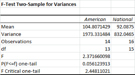
From the above output, the F- test statistic value is 2.37 and its p-value is 0.056.
Decision Rule:
If the p-value is less than the level of significance, reject the null hypothesis. Otherwise, fail to reject the null hypothesis.
Conclusion:
The significance level is 0.05. The p-value is 0.056 and it is greater than the significance level. The null hypothesis is rejected at the 0.05 significance level.
Thus, there is no difference in the variance in team salary among Country A and National league teams.
b.
Create a variable that classifies a team’s total attendance into three groups.
Find whether there is a difference in the
b.
Answer to Problem 50DE
There is no difference in the mean number of games won among the three groups.
Explanation of Solution
Let X represent the total attendance into three groups. Samples 1, 2, and 3 are “less than 2 (million)”, 2 up to 3, and 3 or more attendance of teams of three groups, respectively.
The following table gives the number of games won by the three groups of attendances.
| Sample 1 | Sample 2 | Sample 3 |
| 85 | 81 | 69 |
| 68 | 94 | 88 |
| 55 | 93 | 89 |
| 72 | 61 | 86 |
| 94 | 97 | 74 |
| 75 | 64 | 81 |
| 69 | 94 | |
| 83 | 88 | |
| 66 | 93 | |
| 95 | ||
| 79 | ||
| 76 | ||
| 73 | ||
| 98 |
The null and alternative hypotheses are as follows:
Null hypothesis: There is no difference in the mean number of games won among the three groups.
Alternative hypothesis: There is a difference in the mean number of games won among the three groups
Step-by-step procedure to obtain the test statistic using Excel:
- In Sample 1, enter the number of games won by the team, which is less than 2 million attendances.
- In Sample 2, enter the number of games won by the team of 2 up to 3 million attendances.
- In Sample 3, enter the number of games won by the team of 3 or more million attendances.
- Select the Data tab on the top menu.
- Select Data Analysis and Click on: ANOVA: Single factor and then click on OK.
- In the dialog box, select Input Range.
- Click OK
Output obtained using Excel is represented as follows:
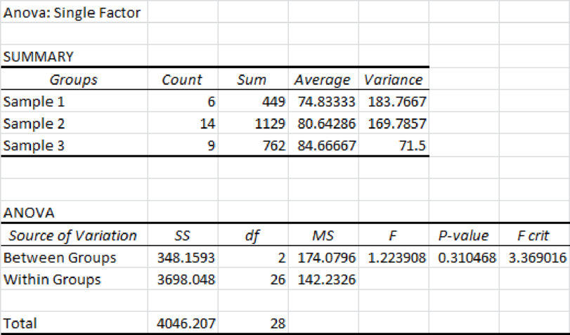
From the above output, the F test statistic value is 1.22 and the p-value is 0.31.
Conclusion:
The level of significance is 0.05. The p-value is greater than the significance level. Hence, one can fail to reject the null hypothesis at the 0.05 significance level. Thus, there is no difference in the mean number of games won among the three groups.
c.
Find whether there is a difference in the mean number of home runs hit per team using the variable defined in Part b.
c.
Answer to Problem 50DE
There is no difference in the mean number of home runs hit per team.
Explanation of Solution
The null and alternative hypotheses are stated below:
Null hypothesis: There is no difference in the mean number of home runs hit per team.
Alternative hypothesis: There is a difference in the mean number of home runs hit per team.
The following table gives the number of home runs per each team, which is defined in Part b.
| Sample 1 | Sample 2 | Sample 3 |
| 211 | 165 | 165 |
| 136 | 149 | 163 |
| 146 | 214 | 187 |
| 131 | 137 | 116 |
| 195 | 172 | 245 |
| 149 | 166 | 158 |
| 175 | 137 | 103 |
| 202 | 159 | |
| 131 | 200 | |
| 139 | ||
| 170 | ||
| 121 | ||
| 198 | ||
| 194 |
Step-by-step procedure to obtain the test statistic using Excel:
- In Sample 1, enter the number of home runs hit by the group of less than 2 million attendances.
- In Sample 2, enter the number of home runs hit by the group of 2 up to 3 million attendances.
- In Sample 3, enter the number of home runs hit by the group of 3 or more million attendances.
- Select the Data tab on the top menu.
- Select Data Analysis and Click on: ANOVA: Single factor and then click on OK.
- In the dialog box, select Input Range.
- Click OK
Output obtained using Excel is represented as follows:
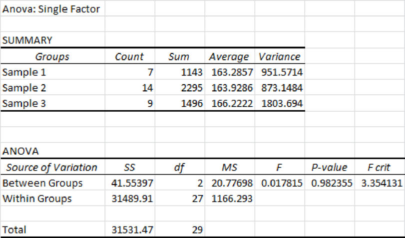
From the above output, the F test statistic value is 0.018 and the p-value is 0.9823.
Conclusion:
The level of significance is 0.05 and the p-value is greater than the significance level. Hence, one fails to reject the null hypothesis at the 0.05 significance level. Thus, there is no difference in the mean number of home runs hit per team.
d.
Find whether there is a difference in the mean salary of the three groups.
d.
Answer to Problem 50DE
The mean salaries are different for each group.
Explanation of Solution
The null and alternative hypotheses are stated below:
Null hypothesis: The mean salary of the three groups is equal.
Alternative hypothesis: At least one mean salary is different from other.
The following table provides the salary of each group that is defined in Part b.
| Sample 1 | Sample 2 | Sample 3 |
| 96.9 | 74.3 | 173.2 |
| 78.4 | 83.3 | 132.3 |
| 60.7 | 81.4 | 154.5 |
| 60.9 | 88.2 | 95.1 |
| 55.4 | 82.2 | 198 |
| 82 | 78.1 | 174.5 |
| 64.2 | 118.1 | 117.6 |
| 97.7 | 110.3 | |
| 94.1 | 120.5 | |
| 93.4 | ||
| 63.4 | ||
| 55.2 | ||
| 75.5 | ||
| 81.3 |
Step-by-step procedure to obtain the test statistic using Excel:
- In Sample 1, enter the salary of the group of less than 2 million attendances.
- In Sample 2, enter the salary of the group of 2 up to 3 million attendances.
- In Sample 3, enter the salary of the group of 3 or more million attendances.
- Select the Data tab on the top menu.
- Select Data Analysis and Click on: ANOVA: Single factor and then click on OK.
- In the dialog box, select Input Range.
- Click OK
Output obtained using Excel is represented as follows:
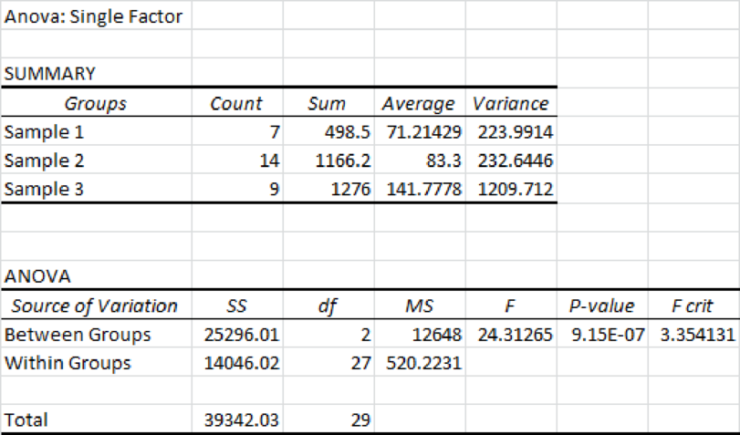
From the above output, the F test statistic value is 24.31 and the p-value is 0.
Conclusion:
The level of significance is 0.05 and the p-value is less than the significance level. Hence, one can reject the null hypothesis at the 0.05 significance level. Thus, the mean salaries are different for each group.
Want to see more full solutions like this?
Chapter 12 Solutions
STATISTICAL TECHNIQUES-ACCESS ONLY


- If, based on a sample size of 900,a political candidate finds that 509people would vote for him in a two-person race, what is the 95%confidence interval for his expected proportion of the vote? Would he be confident of winning based on this poll? Question content area bottom Part 1 A 9595% confidence interval for his expected proportion of the vote is (Use ascending order. Round to four decimal places as needed.)arrow_forwardQuestions An insurance company's cumulative incurred claims for the last 5 accident years are given in the following table: Development Year Accident Year 0 2018 1 2 3 4 245 267 274 289 292 2019 255 276 288 294 2020 265 283 292 2021 263 278 2022 271 It can be assumed that claims are fully run off after 4 years. The premiums received for each year are: Accident Year Premium 2018 306 2019 312 2020 318 2021 326 2022 330 You do not need to make any allowance for inflation. 1. (a) Calculate the reserve at the end of 2022 using the basic chain ladder method. (b) Calculate the reserve at the end of 2022 using the Bornhuetter-Ferguson method. 2. Comment on the differences in the reserves produced by the methods in Part 1.arrow_forwardA population that is uniformly distributed between a=0and b=10 is given in sample sizes 50( ), 100( ), 250( ), and 500( ). Find the sample mean and the sample standard deviations for the given data. Compare your results to the average of means for a sample of size 10, and use the empirical rules to analyze the sampling error. For each sample, also find the standard error of the mean using formula given below. Standard Error of the Mean =sigma/Root Complete the following table with the results from the sampling experiment. (Round to four decimal places as needed.) Sample Size Average of 8 Sample Means Standard Deviation of 8 Sample Means Standard Error 50 100 250 500arrow_forward
- A survey of 250250 young professionals found that two dash thirdstwo-thirds of them use their cell phones primarily for e-mail. Can you conclude statistically that the population proportion who use cell phones primarily for e-mail is less than 0.720.72? Use a 95% confidence interval. Question content area bottom Part 1 The 95% confidence interval is left bracket nothing comma nothing right bracket0.60820.6082, 0.72510.7251. As 0.720.72 is within the limits of the confidence interval, we cannot conclude that the population proportion is less than 0.720.72. (Use ascending order. Round to four decimal places as needed.)arrow_forwardI need help with this problem and an explanation of the solution for the image described below. (Statistics: Engineering Probabilities)arrow_forwardA survey of 250 young professionals found that two-thirds of them use their cell phones primarily for e-mail. Can you conclude statistically that the population proportion who use cell phones primarily for e-mail is less than 0.72? Use a 95% confidence interval. Question content area bottom Part 1 The 95% confidence interval is [ ], [ ] As 0.72 is ▼ above the upper limit within the limits below the lower limit of the confidence interval, we ▼ can cannot conclude that the population proportion is less than 0.72. (Use ascending order. Round to four decimal places as needed.)arrow_forward
- I need help with this problem and an explanation of the solution for the image described below. (Statistics: Engineering Probabilities)arrow_forwardI need help with this problem and an explanation of the solution for the image described below. (Statistics: Engineering Probabilities)arrow_forwardI need help with this problem and an explanation of the solution for the image described below. (Statistics: Engineering Probabilities)arrow_forward
- Questions An insurance company's cumulative incurred claims for the last 5 accident years are given in the following table: Development Year Accident Year 0 2018 1 2 3 4 245 267 274 289 292 2019 255 276 288 294 2020 265 283 292 2021 263 278 2022 271 It can be assumed that claims are fully run off after 4 years. The premiums received for each year are: Accident Year Premium 2018 306 2019 312 2020 318 2021 326 2022 330 You do not need to make any allowance for inflation. 1. (a) Calculate the reserve at the end of 2022 using the basic chain ladder method. (b) Calculate the reserve at the end of 2022 using the Bornhuetter-Ferguson method. 2. Comment on the differences in the reserves produced by the methods in Part 1.arrow_forwardQuestions An insurance company's cumulative incurred claims for the last 5 accident years are given in the following table: Development Year Accident Year 0 2018 1 2 3 4 245 267 274 289 292 2019 255 276 288 294 2020 265 283 292 2021 263 278 2022 271 It can be assumed that claims are fully run off after 4 years. The premiums received for each year are: Accident Year Premium 2018 306 2019 312 2020 318 2021 326 2022 330 You do not need to make any allowance for inflation. 1. (a) Calculate the reserve at the end of 2022 using the basic chain ladder method. (b) Calculate the reserve at the end of 2022 using the Bornhuetter-Ferguson method. 2. Comment on the differences in the reserves produced by the methods in Part 1.arrow_forwardFrom a sample of 26 graduate students, the mean number of months of work experience prior to entering an MBA program was 34.67. The national standard deviation is known to be18 months. What is a 90% confidence interval for the population mean? Question content area bottom Part 1 A 9090% confidence interval for the population mean is left bracket nothing comma nothing right bracketenter your response here,enter your response here. (Use ascending order. Round to two decimal places as needed.)arrow_forward
 Big Ideas Math A Bridge To Success Algebra 1: Stu...AlgebraISBN:9781680331141Author:HOUGHTON MIFFLIN HARCOURTPublisher:Houghton Mifflin Harcourt
 Glencoe Algebra 1, Student Edition, 9780079039897...AlgebraISBN:9780079039897Author:CarterPublisher:McGraw Hill
 Holt Mcdougal Larson Pre-algebra: Student Edition...AlgebraISBN:9780547587776Author:HOLT MCDOUGALPublisher:HOLT MCDOUGAL