
Videos
To test: the null hypothesis and show that it is rejected at the
Explanation of Solution
Given information :
Concept Involved:
In order to decide whether the presumed hypothesis for data sample stands accurate for the entire population or not we use the hypothesis testing.
The critical value from Table A.4, using degrees of freedom of
The values of two qualitative variables are connected and denoted in a contingency table.
This table consists of rows and column. The variables in each row and each column of the table represent a category. The number of rows of contingency table is represented by letter ‘r’ and number of column of contingency table is represented by letter ‘c’.
The formula to find the number of degree of freedom of contingency table is
Calculation:
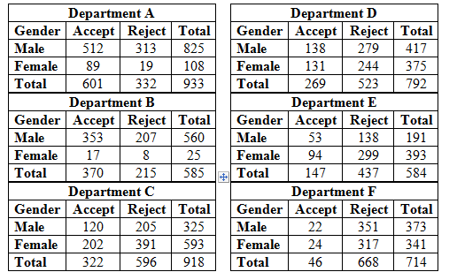
For department A:
| Department A | |||
| Gender | Accept | Reject | Total |
| Male | 512 | 313 | 825 |
| Female | 89 | 19 | 108 |
| Total | 601 | 332 | 933 |
| Finding the expected frequency for the cell corresponding to: | The expected frequency |
| Number of male applicants acceptedin department A The row total is 825, the column total is 601, and the grand total is 933. | |
| Number of male applicants rejectedin department A The row total is 825, the column total is 332, and the grand total is 933. | |
| Number of female applicantsaccepted in department A The row total is 108, the column total is 601, and the grand total is 933. | |
| Number of female applicantsrejected in department A The row total is 108, the column total is 332, and the grand total is 933. |
| Finding the value of the chi-square corresponding to: | |
| Number of male applicants acceptedin department A The observed frequency is 512 and expected frequency is 531.43 | |
| Number of male applicants rejectedin department A The observed frequency is 313 and expected frequency is 293.57 | |
| Number of female applicantsaccepted in department A The observed frequency is 89 and expected frequency is 69.57 | |
| Number of female applicantsrejected in department A The observed frequency is 19 and expected frequency is 38.43 |
To compute the test statistics, we use the observed frequencies and expected frequency:
In department A, % of male accepted =
For department B:
| Department B | |||
| Gender | Accept | Reject | Total |
| Male | 353 | 207 | 560 |
| Female | 17 | 8 | 25 |
| Total | 370 | 215 | 585 |
| Finding the expected frequency for the cell corresponding to: | The expected frequency |
| Number of male applicants acceptedin department B The row total is 560, the column total is 370, and the grand total is 585. | |
| Number of male applicants rejectedin department B The row total is 560, the column total is 215, and the grand total is 585. | |
| Number of female applicantsaccepted in department B The row total is 25, the column total is 370, and the grand total is 585. | |
| Number of female applicantsrejected in department B The row total is 25, the column total is 215, and the grand total is 585. |
| Finding the value of the chi-square corresponding to: | |
| Number of male applicants acceptedin department B The observed frequency is 353 and expected frequency is 354.19 | |
| Number of male applicants rejectedin department B The observed frequency is 207 and expected frequency is 205.81 | |
| Number of female applicantsaccepted in department B The observed frequency is 17 and expected frequency is 15.81 | |
| Number of female applicantsrejected in department B The observed frequency is 8 and expected frequency is 9.19 |
To compute the test statistics, we use the observed frequencies and expected frequency:
In department B, % of male accepted =
For department C:
| Department C | |||
| Gender | Accept | Reject | Total |
| Male | 120 | 205 | 325 |
| Female | 202 | 391 | 593 |
| Total | 322 | 596 | 918 |
| Finding the expected frequency for the cell corresponding to: | The expected frequency |
| Number of male applicants acceptedin department C The row total is 325, the column total is 322, and the grand total is 918. | |
| Number of male applicants rejectedin department C The row total is 325, the column total is 596, and the grand total is918. | |
| Number of female applicantsaccepted in department C The row total is 593, the column total is 322, and the grand total is 918. | |
| Number of female applicantsrejected in department C The row total is 593, the column total is 596, and the grand total is 918. |
| Finding the value of the chi-square corresponding to: | |
| Number of male applicants acceptedin department C The observed frequency is 120 and expected frequency is 114 | |
| Number of male applicants rejectedin department C The observed frequency is 205 and expected frequency is 211 | |
| Number of female applicantsaccepted in department C The observed frequency is 202 and expected frequency is 208 | |
| Number of female applicantsrejected in department C The observed frequency is 391 and expected frequency is 385 |
To compute the test statistics, we use the observed frequencies and expected frequency:
In department C, % of male accepted =
For department D:
| Department D | |||
| Gender | Accept | Reject | Total |
| Male | 138 | 279 | 417 |
| Female | 131 | 244 | 375 |
| Total | 269 | 523 | 792 |
| Finding the expected frequency for the cell corresponding to: | The expected frequency |
| Number of male applicants acceptedin department D The row total is 417, the column total is 269, and the grand total is 792. | |
| Number of male applicants rejectedin department D The row total is 417, the column total is 523, and the grand total is792. | |
| Number of female applicantsaccepted in department D The row total is 375, the column total is 269, and the grand total is 792. | |
| Number of female applicantsrejected in department D The row total is 375, the column total is 523, and the grand total is 792. |
| Finding the value of the chi-square corresponding to: | |
| Number of male applicants acceptedin department D The observed frequency is 138 and expected frequency is 141.63 | |
| Number of male applicants rejectedin department D The observed frequency is 279 and expected frequency is 275.37 | |
| Number of female applicantsaccepted in department D The observed frequency is 131 and expected frequency is 127.37 | |
| Number of female applicantsrejected in department D The observed frequency is 244 and expected frequency is 247.63 |
To compute the test statistics, we use the observed frequencies and expected frequency:
In department D, % of male accepted =
For department E:
| Department E | |||
| Gender | Accept | Reject | Total |
| Male | 53 | 138 | 191 |
| Female | 94 | 299 | 393 |
| Total | 147 | 437 | 584 |
| Finding the expected frequency for the cell corresponding to: | The expected frequency |
| Number of male applicants acceptedin department E The row total is 191, the column total is 147, and the grand total is 584. | |
| Number of male applicants rejectedin department E The row total is 191, the column total is 437, and the grand total is584. | |
| Number of female applicantsaccepted in department E The row total is 393, the column total is 147, and the grand total is 584. | |
| Number of female applicantsrejected in department E The row total is 393, the column total is 437, and the grand total is 584. |
| Finding the value of the chi-square corresponding to: | |
| Number of male applicants acceptedin department E The observed frequency is 53 and expected frequency is 48.08 | |
| Number of male applicants rejectedin department E The observed frequency is 138 and expected frequency is 142.92 | |
| Number of female applicantsaccepted in department E The observed frequency is 94 and expected frequency is 98.92 | |
| Number of female applicantsrejected in department E The observed frequency is 299 and expected frequency is 294.08 |
To compute the test statistics, we use the observed frequencies and expected frequency:
In department E, % of male accepted =
For department F:
| Department F | |||
| Gender | Accept | Reject | Total |
| Male | 22 | 351 | 373 |
| Female | 24 | 317 | 341 |
| Total | 46 | 668 | 714 |
| Finding the expected frequency for the cell corresponding to: | The expected frequency |
| Number of male applicants acceptedin department F The row total is 373, the column total is 46, and the grand total is 714. | |
| Number of male applicants rejectedin department F The row total is 373, the column total is 668, and the grand total is714. | |
| Number of female applicantsaccepted in department F The row total is 341, the column total is 46, and the grand total is 714. | |
| Number of female applicantsrejected in department F The row total is 341, the column total is 668, and the grand total is 714. |
| Finding the value of the chi-square corresponding to: | |
| Number of male applicants acceptedin department F The observed frequency is 22 and expected frequency is 24.03 | |
| Number of male applicants rejectedin department F The observed frequency is 351 and expected frequency is 348.97 | |
| Number of female applicantsaccepted in department F The observed frequency is 24 and expected frequency is 21.97 | |
| Number of female applicantsrejected in department F The observed frequency is 317 and expected frequency is 319.03 |
To compute the test statistics, we use the observed frequencies and expected frequency:
In department E, % of male accepted =
Here r represents the number of rows and c represents the number of columns.
For all the contingency table
| Degrees of freedom | Table A.4 Critical Values for the chi-square Distribution | |||||||||
| 0.995 | 0.99 | 0.975 | 0.95 | 0.90 | 0.10 | 0.05 | 0.025 | 0.01 | 0.005 | |
| 1 | 0.000 | 0.000 | 0.001 | 0.004 | 0.016 | 2.706 | 3.841 | 5.024 | 6.635 | 7.879 |
| 2 | 0.010 | 0.020 | 0.051 | 0.103 | 0.211 | 4.605 | 5.991 | 7.378 | 9.210 | 10.597 |
| 3 | 0.072 | 0.115 | 0.216 | 0.352 | 0.584 | 6.251 | 7.815 | 9.348 | 11.345 | 12.838 |
| 4 | 0.207 | 0.297 | 0.484 | 0.711 | 1.064 | 7.779 | 9.488 | 11.143 | 13.277 | 14.860 |
| 5 | 0.412 | 0.554 | 0.831 | 1.145 | 1.610 | 9.236 | 11.070 | 12.833 | 15.086 | 16.750 |
The critical value is same for all the contingency table.
Conclusion:
For department A:
Test statistic: 17.25; Critical value: 6.635.
For department B:
Test statistic: 0.25; Critical value: 6.635.
For department C:
Test statistic: 0.75; Critical value: 6.635.
For department D:
Test statistic: 0.30; Critical value: 6.635.
For department E:
Test statistic: 1.00; Critical value: 6.635.
For department F:
Test statistic: 0.39; Critical value: 6.635.
In departmentA, 82.4% of the women were accepted, but only 62.1% of themen were accepted.
Want to see more full solutions like this?
Chapter 12 Solutions
Elementary Statistics ( 3rd International Edition ) Isbn:9781260092561


- Business discussarrow_forwardAnalyze the residuals of a linear regression model and select the best response. yes, the residual plot does not show a curve no, the residual plot shows a curve yes, the residual plot shows a curve no, the residual plot does not show a curve I answered, "No, the residual plot shows a curve." (and this was incorrect). I am not sure why I keep getting these wrong when the answer seems obvious. Please help me understand what the yes and no references in the answer.arrow_forwarda. Find the value of A.b. Find pX(x) and py(y).c. Find pX|y(x|y) and py|X(y|x)d. Are x and y independent? Why or why not?arrow_forward
- Analyze the residuals of a linear regression model and select the best response.Criteria is simple evaluation of possible indications of an exponential model vs. linear model) no, the residual plot does not show a curve yes, the residual plot does not show a curve yes, the residual plot shows a curve no, the residual plot shows a curve I selected: yes, the residual plot shows a curve and it is INCORRECT. Can u help me understand why?arrow_forwardYou have been hired as an intern to run analyses on the data and report the results back to Sarah; the five questions that Sarah needs you to address are given below. please do it step by step on excel Does there appear to be a positive or negative relationship between price and screen size? Use a scatter plot to examine the relationship. Determine and interpret the correlation coefficient between the two variables. In your interpretation, discuss the direction of the relationship (positive, negative, or zero relationship). Also discuss the strength of the relationship. Estimate the relationship between screen size and price using a simple linear regression model and interpret the estimated coefficients. (In your interpretation, tell the dollar amount by which price will change for each unit of increase in screen size). Include the manufacturer dummy variable (Samsung=1, 0 otherwise) and estimate the relationship between screen size, price and manufacturer dummy as a multiple…arrow_forwardHere is data with as the response variable. x y54.4 19.124.9 99.334.5 9.476.6 0.359.4 4.554.4 0.139.2 56.354 15.773.8 9-156.1 319.2Make a scatter plot of this data. Which point is an outlier? Enter as an ordered pair, e.g., (x,y). (x,y)= Find the regression equation for the data set without the outlier. Enter the equation of the form mx+b rounded to three decimal places. y_wo= Find the regression equation for the data set with the outlier. Enter the equation of the form mx+b rounded to three decimal places. y_w=arrow_forward
- You have been hired as an intern to run analyses on the data and report the results back to Sarah; the five questions that Sarah needs you to address are given below. please do it step by step Does there appear to be a positive or negative relationship between price and screen size? Use a scatter plot to examine the relationship. Determine and interpret the correlation coefficient between the two variables. In your interpretation, discuss the direction of the relationship (positive, negative, or zero relationship). Also discuss the strength of the relationship. Estimate the relationship between screen size and price using a simple linear regression model and interpret the estimated coefficients. (In your interpretation, tell the dollar amount by which price will change for each unit of increase in screen size). Include the manufacturer dummy variable (Samsung=1, 0 otherwise) and estimate the relationship between screen size, price and manufacturer dummy as a multiple linear…arrow_forwardExercises: Find all the whole number solutions of the congruence equation. 1. 3x 8 mod 11 2. 2x+3= 8 mod 12 3. 3x+12= 7 mod 10 4. 4x+6= 5 mod 8 5. 5x+3= 8 mod 12arrow_forwardScenario Sales of products by color follow a peculiar, but predictable, pattern that determines how many units will sell in any given year. This pattern is shown below Product Color 1995 1996 1997 Red 28 42 21 1998 23 1999 29 2000 2001 2002 Unit Sales 2003 2004 15 8 4 2 1 2005 2006 discontinued Green 26 39 20 22 28 14 7 4 2 White 43 65 33 36 45 23 12 Brown 58 87 44 48 60 Yellow 37 56 28 31 Black 28 42 21 Orange 19 29 Purple Total 28 42 21 49 68 78 95 123 176 181 164 127 24 179 Questions A) Which color will sell the most units in 2007? B) Which color will sell the most units combined in the 2007 to 2009 period? Please show all your analysis, leave formulas in cells, and specify any assumptions you make.arrow_forward
- One hundred students were surveyed about their preference between dogs and cats. The following two-way table displays data for the sample of students who responded to the survey. Preference Male Female TOTAL Prefers dogs \[36\] \[20\] \[56\] Prefers cats \[10\] \[26\] \[36\] No preference \[2\] \[6\] \[8\] TOTAL \[48\] \[52\] \[100\] problem 1 Find the probability that a randomly selected student prefers dogs.Enter your answer as a fraction or decimal. \[P\left(\text{prefers dogs}\right)=\] Incorrect Check Hide explanation Preference Male Female TOTAL Prefers dogs \[\blueD{36}\] \[\blueD{20}\] \[\blueE{56}\] Prefers cats \[10\] \[26\] \[36\] No preference \[2\] \[6\] \[8\] TOTAL \[48\] \[52\] \[100\] There were \[\blueE{56}\] students in the sample who preferred dogs out of \[100\] total students.arrow_forwardBusiness discussarrow_forwardYou have been hired as an intern to run analyses on the data and report the results back to Sarah; the five questions that Sarah needs you to address are given below. Does there appear to be a positive or negative relationship between price and screen size? Use a scatter plot to examine the relationship. Determine and interpret the correlation coefficient between the two variables. In your interpretation, discuss the direction of the relationship (positive, negative, or zero relationship). Also discuss the strength of the relationship. Estimate the relationship between screen size and price using a simple linear regression model and interpret the estimated coefficients. (In your interpretation, tell the dollar amount by which price will change for each unit of increase in screen size). Include the manufacturer dummy variable (Samsung=1, 0 otherwise) and estimate the relationship between screen size, price and manufacturer dummy as a multiple linear regression model. Interpret the…arrow_forward
 Big Ideas Math A Bridge To Success Algebra 1: Stu...AlgebraISBN:9781680331141Author:HOUGHTON MIFFLIN HARCOURTPublisher:Houghton Mifflin Harcourt
 Glencoe Algebra 1, Student Edition, 9780079039897...AlgebraISBN:9780079039897Author:CarterPublisher:McGraw Hill
 Functions and Change: A Modeling Approach to Coll...AlgebraISBN:9781337111348Author:Bruce Crauder, Benny Evans, Alan NoellPublisher:Cengage Learning
 Holt Mcdougal Larson Pre-algebra: Student Edition...AlgebraISBN:9780547587776Author:HOLT MCDOUGALPublisher:HOLT MCDOUGAL