(a)
To find: The expression of contrast for each of the treatments in terms of their respective means.
(a)
Answer to Problem 49E
Solution: The expression of contrast for the experiment including the treatment of Placebo verses average of two low dose treatment is given below:
The expression of contrast for the experiment including the treatment of difference between high A and low A verses high B and low B is given below:
Explanation of Solution
Calculation: The average of means of low A and low B treatment is
Null hypotheses represent that there is no difference in the Placebo treatment and average of low A and low B treatment, which is represented as below:
Hence, on equating
The difference of means of low A and high A treatment is
Null hypotheses represent that there is no difference in the difference of low A and high A treatment and difference of high B and low B treatment, which is represented as below:
Hence, on equating
The coefficients of contrast for the contrast
The coefficients of contrast for the contrast
(b)
To find: The sample and standard error for each of the contrast.
(b)
Answer to Problem 49E
Solution: The sample of contrast
The standard error for the contrast
Explanation of Solution
Calculation: The value of contrast
The value of contrast
Standard error can be calculated by using the formula given below:
Pooled standard deviation can be calculated as given below:
For the first contrast, the standard error
For the second contrast, the standard error
Interpretation: Therefore, it can be concluded that for the first contrast, the estimated value of standard deviation is 2.1353 and for the second contrast, the estimated value of standard deviation is 3.487.
(c)
To test: The significance test for each of the contrast and summarize the obtained results.
(c)
Answer to Problem 49E
Solution: The test statistic for contrast of the experiment including the treatment of Placebo verses average of two low dose treatment is 0.0414 and the test statistics for contrast for the experiment including the treatment of difference between high A and low A verses high B and low B is 0.2540. For the first contrast, the result is significant but for the second contrast the result is insignificant.
Explanation of Solution
Calculation: Test statistic can be calculated by using following formula, which is mentioned below:
To calculate the test statistic for first contrast, the value of
The total
The degree of freedom for contrast can be obtained as shown below:
The P-value can also be calculated by the software Microsoft Excel by using the following command:
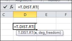
Insert the values of x and degree of freedom, which are –1.8264 and 20, respectively. After this, press enter and the output is shown below in the snapshot:
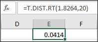
Hence, the P- value is obtained as 0.0414, which is less than the significance level 0.05, so the decision is to reject the null hypothesis.
To calculate the test statistic for second contrast, the value of
The P-value can also be calculated by the software Microsoft Excel by using the following command:
Insert the values of x and degree of freedom, which is 0.6739 and 20, respectively. After this, press enter and the output is shown below in the snapshot:
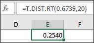
Hence, the P- value is obtained as 0.2540, which is greater than the significance level 0.05, so the decision is to accept the null hypothesis.
Conclusion: Therefore, it can be concluded that the result is significant for the first contrast and the result is not significant for the second contrast.
Want to see more full solutions like this?
Chapter 12 Solutions
LaunchPad for Moore's Introduction to the Practice of Statistics (12 month access)

- ian income of $50,000. erty rate of 13. Using data from 50 workers, a researcher estimates Wage = Bo+B,Education + B₂Experience + B3Age+e, where Wage is the hourly wage rate and Education, Experience, and Age are the years of higher education, the years of experience, and the age of the worker, respectively. A portion of the regression results is shown in the following table. ni ogolloo bash 1 Standard Coefficients error t stat p-value Intercept 7.87 4.09 1.93 0.0603 Education 1.44 0.34 4.24 0.0001 Experience 0.45 0.14 3.16 0.0028 Age -0.01 0.08 -0.14 0.8920 a. Interpret the estimated coefficients for Education and Experience. b. Predict the hourly wage rate for a 30-year-old worker with four years of higher education and three years of experience.arrow_forward1. If a firm spends more on advertising, is it likely to increase sales? Data on annual sales (in $100,000s) and advertising expenditures (in $10,000s) were collected for 20 firms in order to estimate the model Sales = Po + B₁Advertising + ε. A portion of the regression results is shown in the accompanying table. Intercept Advertising Standard Coefficients Error t Stat p-value -7.42 1.46 -5.09 7.66E-05 0.42 0.05 8.70 7.26E-08 a. Interpret the estimated slope coefficient. b. What is the sample regression equation? C. Predict the sales for a firm that spends $500,000 annually on advertising.arrow_forwardCan you help me solve problem 38 with steps im stuck.arrow_forward
- How do the samples hold up to the efficiency test? What percentages of the samples pass or fail the test? What would be the likelihood of having the following specific number of efficiency test failures in the next 300 processors tested? 1 failures, 5 failures, 10 failures and 20 failures.arrow_forwardThe battery temperatures are a major concern for us. Can you analyze and describe the sample data? What are the average and median temperatures? How much variability is there in the temperatures? Is there anything that stands out? Our engineers’ assumption is that the temperature data is normally distributed. If that is the case, what would be the likelihood that the Safety Zone temperature will exceed 5.15 degrees? What is the probability that the Safety Zone temperature will be less than 4.65 degrees? What is the actual percentage of samples that exceed 5.25 degrees or are less than 4.75 degrees? Is the manufacturing process producing units with stable Safety Zone temperatures? Can you check if there are any apparent changes in the temperature pattern? Are there any outliers? A closer look at the Z-scores should help you in this regard.arrow_forwardNeed help pleasearrow_forward
- Please conduct a step by step of these statistical tests on separate sheets of Microsoft Excel. If the calculations in Microsoft Excel are incorrect, the null and alternative hypotheses, as well as the conclusions drawn from them, will be meaningless and will not receive any points. 4. One-Way ANOVA: Analyze the customer satisfaction scores across four different product categories to determine if there is a significant difference in means. (Hints: The null can be about maintaining status-quo or no difference among groups) H0 = H1=arrow_forwardPlease conduct a step by step of these statistical tests on separate sheets of Microsoft Excel. If the calculations in Microsoft Excel are incorrect, the null and alternative hypotheses, as well as the conclusions drawn from them, will be meaningless and will not receive any points 2. Two-Sample T-Test: Compare the average sales revenue of two different regions to determine if there is a significant difference. (Hints: The null can be about maintaining status-quo or no difference among groups; if alternative hypothesis is non-directional use the two-tailed p-value from excel file to make a decision about rejecting or not rejecting null) H0 = H1=arrow_forwardPlease conduct a step by step of these statistical tests on separate sheets of Microsoft Excel. If the calculations in Microsoft Excel are incorrect, the null and alternative hypotheses, as well as the conclusions drawn from them, will be meaningless and will not receive any points 3. Paired T-Test: A company implemented a training program to improve employee performance. To evaluate the effectiveness of the program, the company recorded the test scores of 25 employees before and after the training. Determine if the training program is effective in terms of scores of participants before and after the training. (Hints: The null can be about maintaining status-quo or no difference among groups; if alternative hypothesis is non-directional, use the two-tailed p-value from excel file to make a decision about rejecting or not rejecting the null) H0 = H1= Conclusion:arrow_forward
- Please conduct a step by step of these statistical tests on separate sheets of Microsoft Excel. If the calculations in Microsoft Excel are incorrect, the null and alternative hypotheses, as well as the conclusions drawn from them, will be meaningless and will not receive any points. The data for the following questions is provided in Microsoft Excel file on 4 separate sheets. Please conduct these statistical tests on separate sheets of Microsoft Excel. If the calculations in Microsoft Excel are incorrect, the null and alternative hypotheses, as well as the conclusions drawn from them, will be meaningless and will not receive any points. 1. One Sample T-Test: Determine whether the average satisfaction rating of customers for a product is significantly different from a hypothetical mean of 75. (Hints: The null can be about maintaining status-quo or no difference; If your alternative hypothesis is non-directional (e.g., μ≠75), you should use the two-tailed p-value from excel file to…arrow_forwardPlease conduct a step by step of these statistical tests on separate sheets of Microsoft Excel. If the calculations in Microsoft Excel are incorrect, the null and alternative hypotheses, as well as the conclusions drawn from them, will be meaningless and will not receive any points. 1. One Sample T-Test: Determine whether the average satisfaction rating of customers for a product is significantly different from a hypothetical mean of 75. (Hints: The null can be about maintaining status-quo or no difference; If your alternative hypothesis is non-directional (e.g., μ≠75), you should use the two-tailed p-value from excel file to make a decision about rejecting or not rejecting null. If alternative is directional (e.g., μ < 75), you should use the lower-tailed p-value. For alternative hypothesis μ > 75, you should use the upper-tailed p-value.) H0 = H1= Conclusion: The p value from one sample t-test is _______. Since the two-tailed p-value is _______ 2. Two-Sample T-Test:…arrow_forwardPlease conduct a step by step of these statistical tests on separate sheets of Microsoft Excel. If the calculations in Microsoft Excel are incorrect, the null and alternative hypotheses, as well as the conclusions drawn from them, will be meaningless and will not receive any points. What is one sample T-test? Give an example of business application of this test? What is Two-Sample T-Test. Give an example of business application of this test? .What is paired T-test. Give an example of business application of this test? What is one way ANOVA test. Give an example of business application of this test? 1. One Sample T-Test: Determine whether the average satisfaction rating of customers for a product is significantly different from a hypothetical mean of 75. (Hints: The null can be about maintaining status-quo or no difference; If your alternative hypothesis is non-directional (e.g., μ≠75), you should use the two-tailed p-value from excel file to make a decision about rejecting or not…arrow_forward
 MATLAB: An Introduction with ApplicationsStatisticsISBN:9781119256830Author:Amos GilatPublisher:John Wiley & Sons Inc
 Probability and Statistics for Engineering and th...StatisticsISBN:9781305251809Author:Jay L. DevorePublisher:Cengage Learning
 Statistics for The Behavioral Sciences (MindTap C...StatisticsISBN:9781305504912Author:Frederick J Gravetter, Larry B. WallnauPublisher:Cengage Learning
 Elementary Statistics: Picturing the World (7th E...StatisticsISBN:9780134683416Author:Ron Larson, Betsy FarberPublisher:PEARSON
 The Basic Practice of StatisticsStatisticsISBN:9781319042578Author:David S. Moore, William I. Notz, Michael A. FlignerPublisher:W. H. Freeman
 Introduction to the Practice of StatisticsStatisticsISBN:9781319013387Author:David S. Moore, George P. McCabe, Bruce A. CraigPublisher:W. H. Freeman