
(a)
The IS curve of the economy.
(a)
Explanation of Solution
The investment function of the economy is given by
The values of C, T, I, and G can be substituted into the IS equation as follows:
Thus, the IS curve of the economy can be graphed by plotting the Y value on the horizontal axis as 3000 and r ranging from 0 to 8 as follows:
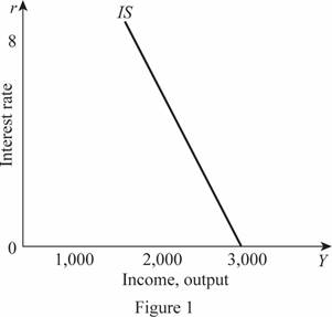
In Figure 1, the horizontal axis measures the income or output and the vertical axis measures the interest rate.
Fiscal policy: The fiscal policy is a policy of the government regarding the government expenditures and taxes of the economy.
(b)
The LM curve of the economy.
(b)
Explanation of Solution
The money demand function of the economy is given to be
The supply of real money balance can be calculated by dividing the money supply by the price level in the economy. Since their values are given, the value of the supply of the real money balance can be calculated as follows:
Thus, the supply of real money balance is 1,000. The LM curve can be calculated by setting the demand equation equal to the supply equation as follows:
Thus, the LM curve with the value of r ranging from 0 to 8 can be plotted as follows:
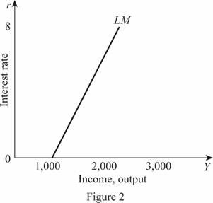
In Figure 2, the horizontal axis measures the income or output and the vertical axis measures the interest rate.
(c)
The IS-LM equilibrium.
(c)
Explanation of Solution
The IS-LM equilibrium can be calculated by equating the IS equation and the LM equation. The IS equation is calculated to be
Substituting the value of r in any equation can provide the value of Y as follows:
Thus, the rate of interest and Y are 5 and 2,000, respectively. These values can be obtained through the graph as follows:
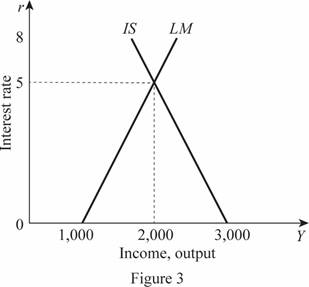
In Figure 3, the horizontal axis measures the income or output and the vertical axis measures the interest rate. The market is in equilibrium at the point where the IS curve intersects with the LM curve.
(d)
The impact of increased government purchases from 500 to 700 on IS and IS-LM equilibrium.
(d)
Explanation of Solution
The values of C, T, I, and G can be substituted into the IS equation as follows:
The new IS curve is 500 more than the previous IS curve, which means that the IS curve will shift toward the right by the value of 500 when the government purchases increases from 500 to 700. Thus, the IS and the LM equations can be equated to calculate the IS-LM equation as follows:
Substituting the value of r in any equation can provide the value of Y as follows:
Thus, the rate of interest and Y are 6.25 and 2,250, respectively. These values can be obtained through the graph as follows:
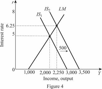
In Figure 4, the horizontal axis measures the income or output and the vertical axis measures the interest rate. Thus, with an increase in the government expenditure from 500 to 700, the IS curve shifts to the right. The equilibrium rate of interest in the economy increases by 1.25 from 5 to 6.25. The change in the income is by $250 and from $2,000, it becomes $2,250.
(e)
The impact of increased money supply from 3000 to 4500 on IS and IS-LM equilibrium.
(e)
Explanation of Solution
The supply of real money balance can be calculated by dividing the money supply by the price level in the economy. Since their values are given, the value of the supply of the real money balance can be calculated as follows:
Thus, the supply of real money balance is 1,500. The LM curve can be calculated by setting the demand equation equal to the supply equation as follows:
Thus, the LM value will change by 500, which means there will be a rightward shift in the LM curve with the value of 500. The rightward shift in the LM curve will lead to the change in the equilibrium and this can be calculated as follows:
Substituting the value of r in any equation can provide the value of Y as follows:
Thus, the rate of interest and Y are 3.75 and 2,250, respectively. These values can be obtained through the graph as follows:
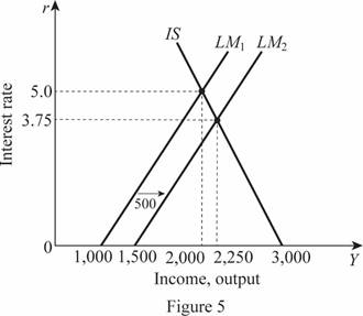
In Figure 5, the horizontal axis measures the income or output and the vertical axis measures the interest rate.
(f)
The impact of increased price level from 3 to 5 on IS and IS-LM equilibrium.
(f)
Explanation of Solution
The supply of real money balance can be calculated by dividing the money supply by the price level in the economy. Since their values are given, the value of the supply of the real money balance can be calculated as follows:
Thus, the supply of real money balance is 600. The LM curve can be calculated by setting the demand equation equal to the supply equation as follows:
Thus, the LM value will change by -400, which means there will be a leftward shift in the LM curve with the value of 400. The leftward shift in the LM curve will lead to the change in the equilibrium and this can be calculated as follows:
Substituting the value of r in any equation can provide the value of Y as follows:
Thus, the rate of interest and Y are 6 and 1,800, respectively. These values can be obtained through the graph as follows:
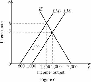
In Figure 6, the horizontal axis measures the income or output and the vertical axis measures the interest rate.
(g)
The impact of changes in the fiscal and monetary policies on aggregate demand.
(g)
Explanation of Solution
The aggregate demand curve is the relationship between the price level in the economy and the level of income of the economy. Thus, the aggregate demand curve can be derived by summating the IS and LM curves and solving it for the value of Y as the function of P. This can be done as follows:
The IS curve can be written in terms of the rate of interest as follows:
Similarly, the LM equation can be written in terms of the rate of interest as follows:
Now, the IS and LM curves can be combined to eliminate the rate of interest and solving the equation for Y as a function of P as follows:
The nominal money supply is given to be 3,000, which can be substituted in the above equation for M and can be calculated as follows:
This aggregate demand equation can be graphed as follows:
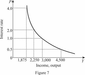
In Figure 7, the horizontal axis measures the income or output and the vertical axis measures the price level. When there is a change in the money supply as well as in the government purchases, the IS curve will be derived with the changed government purchases. This can be calculated as follows:
The IS curve can be written in terms of the rate of interest as follows:
Similarly, the LM equation can be written in terms of the rate of interest as follows:
Now, the IS and LM curves can be combined to eliminate the rate of interest and solving the equation for Y as a function of P as follows:
Thus, the change in the government expenditure with 200 leads to an increase in the aggregate demand with a value of 250. When the expansionary monetary policy increases the money supply from 3,000 to 4,500, the LM curve will change and the new aggregate demand can be calculated as follows:
The normal AD curve is calculated to be
Thus, an increased money supply leads to a rightward shift in the AD curve of the economy.
Want to see more full solutions like this?
Chapter 12 Solutions
MACROECONOMICS+ACHIEVE 1-TERM AC (LL)

- how to caculate verible cost?arrow_forwardWhat is the deficit?arrow_forwardIdentify the two curves shown on the graph, and explain their upward and downward slopes. Why does curve Aintersect the horizontal axis? What is the significance of quantity d? What does erepresent? How would the optimal quantity of information change if the marginal benefit of information increased—that is, if the marginal benefit curve shifted upward?arrow_forward
- 6. Rent seeking The following graph shows the demand, marginal revenue, and marginal cost curves for a single-price monopolist that produces a drug that helps relieve arthritis pain. Place the grey point (star symbol) in the appropriate location on the graph to indicate the monopoly outcome such that the dashed lines reveal the profit-maximizing price and quantity of a single-price monopolist. Then, use the green rectangle (triangle symbols) to show the profits earned by the monopolist. 18 200 20 16 16 14 PRICE (Dollars per dose) 12 10 10 8 4 2 MC = ATC MR Demand 0 0 5 10 15 20 25 30 35 40 45 50 QUANTITY (Millions of doses per year) Monopoly Outcome Monopoly Profits Suppose that should the patent on this particular drug expire, the market would become perfectly competitive, with new firms immediately entering the market with essentially identical products. Further suppose that in this case the original firm will hire lobbyists and make donations to several key politicians to extend its…arrow_forwardConsider a call option on a stock that does not pay dividends. The stock price is $100 per share, and the risk-free interest rate is 10%. The call strike is $100 (at the money). The stock moves randomly with u=2 and d=0.5. 1. Write the system of equations to replicate the option using A shares and B bonds. 2. Solve the system of equations and determine the number of shares and the number of bonds needed to replicate the option. Show your answer with 4 decimal places (x.xxxx); do not round intermediate calculations. This is easy to do in Excel. A = B = 3. Use A shares and B bonds from the prior question to calculate the premium on the option. Again, do not round intermediate calculations and show your answer with 4 decimal places. Call premium =arrow_forwardAnswer these questions using replication or the risk neutral probability. Both methods will produce the same answer. Show your work to receive credit. 6. What is the premium of a call with a higher strike. Show your work to receive credit; do not round intermediate calculations. S0 = $100, u=2, d=0.5, r=10%, strike=$150arrow_forward
- Answer these questions using replication or the risk neutral probability. Both methods will produce the same answer.arrow_forwardProblem 2: At a raffle, 2000 tickets are sold at $5 each for five prizes of $2000, $1000, $500, $250, and $100. You buy one ticket. What is the expected value of your gain? 1. Find the gain for each prize. 2. Write a probability distribution for the possible gains. 3. Find the expected value. 4. Interpret the results.arrow_forwardThis activity focuses on developing direct and supported opinions using various sources of information on the importance of the following topics: non-renewable and renewable energies, economic factors and obstacles that can affect the relationship between international trade and economic growth, devaluation of the currency in countries, and the imbalance of economic equity. In this context, it is essential that, when studying and developing these topics, students understand the concepts of the value of currencies and that leads to devaluation, non-renewable and renewable energy resources, economic development and obstacles, distribution of wealth, economic growth and external and internal constraints, and about international trade as a growth factor. Thus, the objectives that are intended to be achieved are the following: Acquire knowledge about the concepts mentioned above. Determine relationships between economic growth and international trade. Understand what some limitations that…arrow_forward
- Consider a firm facing conventional production technology. The short run Production Function has a small range of increasing marginal product (increasing marginal returns) and then is subject to the Law of Diminishing Marginal Product (diminishing marginal returns). A. Putting quantity on the horizontal axis and dollars on the vertical axis, depict three important curves: Fixed Cost (FC), Variable Cost (VC), and Total Cost (TC). (Note that we are not asking you to depict average cost functions!) B. Please clearly indicate on this graph the range of quantities where the firm is experiencing (1) increasing marginal product and (2) diminishing marginal product. C. In a few sentences, please justify why you've made this specific classification of increasing/diminishing marginal product in part (b).arrow_forwardplease answer the following questions: What is money, and why does anyone want it? Explain the concept of the opportunity cost of holding money . Explain why an increase in U.S. interest rates relative to UK interest rates would affect the U.S.-UK exchange rate. Suppose that a person’s wealth is $50,000 and that her yearlyincome is $60,000. Also suppose that her money demand functionis given by Md = $Y10.35 - i2Derive the demand for bonds. Suppose the interest rate increases by 10 percentage points. What is the effect on her demand for bonds?b. What are the effects of an increase in income on her demand for money and her demand for bonds? Explain in wordsarrow_forwardDriving Quiz X My Course G city place w x D2L Login - Univ X D2L Login - Univ x D2L Login - U acmillanlearning.com/ihub/assessment/f188d950-dd73-11e0-9572-0800200c9a66/4db68a5e-69bb-4767-8d6c-a12d +1687 pts /1800 © Macmillan Learning Question 6 of 18 > The graph shows the average total cost (ATC) curve, the marginal cost (MC) curve, the average variable cost (AVC) curve, and the marginal revenue (MR) curve (which is also the market price) for a perfectly competitive firm that produces terrible towels. Answer the three questions, assuming that the firm is profit-maximizing and does not shut down in the short run. What is the firm's total revenue? S What is the firm's total cost? $ What is the firm's profit? (Enter a negative number for a loss.) $ Price $320 $300 $200 $150 205 260 336 365 Quantity MC ATC AVC MR=Parrow_forward

 Economics (MindTap Course List)EconomicsISBN:9781337617383Author:Roger A. ArnoldPublisher:Cengage Learning


