Chapter 1.2, Problem 1.33E

a)

To determine

To find two sources of variation.

Explanation of Solution

Given:

  

There might be many sources of variations. One of the sources of variation might be the paper towels were not placed in the water the same way. Second source of variation will be the Samantha did not squeeze out all the water in some paper towels. There is evidence available of these sources of variation. These sources of variation can be seen by sometimes very different amounts of water absorbed by each brand of paper towels. So, these sources of variation just provide the different guesses about the cause of same problem.

b)

To determine

To explain four-step statistical problem-solving process.

Explanation of Solution

Given:

  

I) The question of interest: The question can be asked as which brand of paper towel, between Bounty, Scott, Sparkle, and Western Family, is the most absorbent.

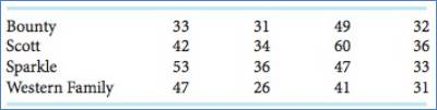
II) Data collection: The data can be generating by one of the experiments. Starting out with four individual sheets of each brand. One a time, one sheet of paper towel was placed to the bottom of a container containing 200 milliliters of water. After some time (20 seconds), the paper towel was removed from the water and all of the water was squeezed out into a graduated cylinder so that the amount of water absorbed could be measured. This was repeated another three times for each brand and this same procedure was repeated for every other brand of paper towel as well. The data will be like:

Brand	Average Absorbance (mL)
Bounty	36.25
Scott	43
Sparkle	42.25
Western Family	36.25

III) Analysis of data: Therefore, average absorbances of each of the paper towels will observed. This will be found to account for the massive variation between the absorbances.

IV) Results: It is observed that Scott brand paper towels are most absorbent, followed closely by Sparkle brand, while Bounty and Western family tie for least absorbent.