
Concept explainers
Videos
Applet Exercise Refer to Exercises 11.2 and 11.5. The data from Exercise 11.5 appear in the graph under the heading “Another Example” in the applet Fitting a Line Using Least Squares. Again, the horizontal blue line that initially appears on the graph is a line with 0 slope.
- a What is the intercept of the line with 0 slope? What is the value of SSE for the line with 0 slope?
- b Do you think that a line with negative slope will fit the data well? If the line is dragged to produce a negative slope, does SSE increase or decrease?
- c Drag the line to obtain a line that visually fits the data well. What is the equation of the line that you obtained? What is the value of SSE? What happens to SSE if the slope (and intercept) of the line is changed from the one that you visually fit?
- d Is the line that you visually fit the least-squares line? Click on the button “Find Best Model” to obtain the line with smallest SSE. How do the slope and intercept of the least-squares line compare to the slope and intercept of the line that you visually fit in part (c)? How do the SSEs compare?
- e Refer to part (a). What is the y-coordinate of the point around which the blue line pivots?
- f Click on the button “Display/Hide Error Squares.” What do you observe about the size of the yellow squares that appear on the graph? What is the sum of the areas of the yellow squares?
11.2 Applet Exercise How can you improve your understanding of what the method of least-squares actually does? Access the applet Fitting a Line Using Least Squares (at academic.cengage.com/statistics/wackerly). The data that appear on the first graph is from Example 11.1.
- a What are the slope and intercept of the blue horizontal line? (See the equation above the graph.) What is the sum of the squares of the vertical deviations between the points on the horizontal line and the observed values of the y’s? Does the horizontal line fit the data well? Click the button “Display/Hide Error Squares.” Notice that the areas of the yellow boxes are equal to the squares of the associated deviations. How does SSE compare to the sum of the areas of the yellow boxes?
- b Click the button “Display/Hide Error Squares” so that the yellow boxes disappear. Place the cursor on right end of the blue line. Click and hold the mouse button and drag the line so that the slope of the blue line becomes negative. What do you notice about the lengths of the vertical red lines? Did SSE increase of decrease? Does the line with negative slope appear to fit the data well?
- c Drag the line so that the slope is near 0.8. What happens as you move the slope closer to 0.7? Did SSE increase or decrease? When the blue line is moved, it is actually pivoting around a fixed point. What are the coordinates of that pivot point? Are the coordinates of the pivot point consistent with the result you derive in Exercise 11.1?
- d Drag the blue line until you obtain a line that visually fits the data well. What are the slope and intercept of the line that you visually fit to the data? What is the value of SSE for the line that you visually fit to the data? Click the button “Find Best Model” to obtain the least-squares line. How does the value of SSE compare to the SSE associated with the line that you visually fit to the data? How do the slope and intercept of the line that you visually fit to the data compare to slope and intercept of the least-squares line?
11.1 If
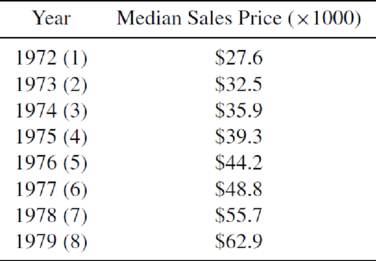
11.5 What did housing prices look like in the “good old days”? The
Want to see the full answer?
Check out a sample textbook solution
Chapter 11 Solutions
Mathematical Statistics with Applications


- A company found that the daily sales revenue of its flagship product follows a normal distribution with a mean of $4500 and a standard deviation of $450. The company defines a "high-sales day" that is, any day with sales exceeding $4800. please provide a step by step on how to get the answers in excel Q: What percentage of days can the company expect to have "high-sales days" or sales greater than $4800? Q: What is the sales revenue threshold for the bottom 10% of days? (please note that 10% refers to the probability/area under bell curve towards the lower tail of bell curve) Provide answers in the yellow cellsarrow_forwardFind the critical value for a left-tailed test using the F distribution with a 0.025, degrees of freedom in the numerator=12, and degrees of freedom in the denominator = 50. A portion of the table of critical values of the F-distribution is provided. Click the icon to view the partial table of critical values of the F-distribution. What is the critical value? (Round to two decimal places as needed.)arrow_forwardA retail store manager claims that the average daily sales of the store are $1,500. You aim to test whether the actual average daily sales differ significantly from this claimed value. You can provide your answer by inserting a text box and the answer must include: Null hypothesis, Alternative hypothesis, Show answer (output table/summary table), and Conclusion based on the P value. Showing the calculation is a must. If calculation is missing,so please provide a step by step on the answers Numerical answers in the yellow cellsarrow_forward
 Glencoe Algebra 1, Student Edition, 9780079039897...AlgebraISBN:9780079039897Author:CarterPublisher:McGraw Hill
 Big Ideas Math A Bridge To Success Algebra 1: Stu...AlgebraISBN:9781680331141Author:HOUGHTON MIFFLIN HARCOURTPublisher:Houghton Mifflin Harcourt
 Linear Algebra: A Modern IntroductionAlgebraISBN:9781285463247Author:David PoolePublisher:Cengage Learning
 Elementary Linear Algebra (MindTap Course List)AlgebraISBN:9781305658004Author:Ron LarsonPublisher:Cengage Learning
 Algebra: Structure And Method, Book 1AlgebraISBN:9780395977224Author:Richard G. Brown, Mary P. Dolciani, Robert H. Sorgenfrey, William L. ColePublisher:McDougal Littell