Concept explainers
Videos
Applet Exercise Refer to Exercises 11.2 and 11.5. The data from Exercise 11.5 appear in the graph under the heading “Another Example” in the applet Fitting a Line Using Least Squares. Again, the horizontal blue line that initially appears on the graph is a line with 0 slope.
- a What is the intercept of the line with 0 slope? What is the value of SSE for the line with 0 slope?
- b Do you think that a line with negative slope will fit the data well? If the line is dragged to produce a negative slope, does SSE increase or decrease?
- c Drag the line to obtain a line that visually fits the data well. What is the equation of the line that you obtained? What is the value of SSE? What happens to SSE if the slope (and intercept) of the line is changed from the one that you visually fit?
- d Is the line that you visually fit the least-squares line? Click on the button “Find Best Model” to obtain the line with smallest SSE. How do the slope and intercept of the least-squares line compare to the slope and intercept of the line that you visually fit in part (c)? How do the SSEs compare?
- e Refer to part (a). What is the y-coordinate of the point around which the blue line pivots?
- f Click on the button “Display/Hide Error Squares.” What do you observe about the size of the yellow squares that appear on the graph? What is the sum of the areas of the yellow squares?
11.2 Applet Exercise How can you improve your understanding of what the method of least-squares actually does? Access the applet Fitting a Line Using Least Squares (at academic.cengage.com/statistics/wackerly). The data that appear on the first graph is from Example 11.1.
- a What are the slope and intercept of the blue horizontal line? (See the equation above the graph.) What is the sum of the squares of the vertical deviations between the points on the horizontal line and the observed values of the y’s? Does the horizontal line fit the data well? Click the button “Display/Hide Error Squares.” Notice that the areas of the yellow boxes are equal to the squares of the associated deviations. How does SSE compare to the sum of the areas of the yellow boxes?
- b Click the button “Display/Hide Error Squares” so that the yellow boxes disappear. Place the cursor on right end of the blue line. Click and hold the mouse button and drag the line so that the slope of the blue line becomes negative. What do you notice about the lengths of the vertical red lines? Did SSE increase of decrease? Does the line with negative slope appear to fit the data well?
- c Drag the line so that the slope is near 0.8. What happens as you move the slope closer to 0.7? Did SSE increase or decrease? When the blue line is moved, it is actually pivoting around a fixed point. What are the coordinates of that pivot point? Are the coordinates of the pivot point consistent with the result you derive in Exercise 11.1?
- d Drag the blue line until you obtain a line that visually fits the data well. What are the slope and intercept of the line that you visually fit to the data? What is the value of SSE for the line that you visually fit to the data? Click the button “Find Best Model” to obtain the least-squares line. How does the value of SSE compare to the SSE associated with the line that you visually fit to the data? How do the slope and intercept of the line that you visually fit to the data compare to slope and intercept of the least-squares line?
11.1 If
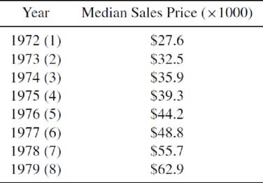
11.5 What did housing prices look like in the “good old days”? The
Want to see the full answer?
Check out a sample textbook solution
Chapter 11 Solutions
Mathematical Statistics with Applications


- For each of the time series, construct a line chart of the data and identify the characteristics of the time series (that is, random, stationary, trend, seasonal, or cyclical). Year Month Rate (%)2009 Mar 8.72009 Apr 9.02009 May 9.42009 Jun 9.52009 Jul 9.52009 Aug 9.62009 Sep 9.82009 Oct 10.02009 Nov 9.92009 Dec 9.92010 Jan 9.82010 Feb 9.82010 Mar 9.92010 Apr 9.92010 May 9.62010 Jun 9.42010 Jul 9.52010 Aug 9.52010 Sep 9.52010 Oct 9.52010 Nov 9.82010 Dec 9.32011 Jan 9.12011 Feb 9.02011 Mar 8.92011 Apr 9.02011 May 9.02011 Jun 9.12011 Jul 9.02011 Aug 9.02011 Sep 9.02011 Oct 8.92011 Nov 8.62011 Dec 8.52012 Jan 8.32012 Feb 8.32012 Mar 8.22012 Apr 8.12012 May 8.22012 Jun 8.22012 Jul 8.22012 Aug 8.12012 Sep 7.82012 Oct…arrow_forwardFor each of the time series, construct a line chart of the data and identify the characteristics of the time series (that is, random, stationary, trend, seasonal, or cyclical). Date IBM9/7/2010 $125.959/8/2010 $126.089/9/2010 $126.369/10/2010 $127.999/13/2010 $129.619/14/2010 $128.859/15/2010 $129.439/16/2010 $129.679/17/2010 $130.199/20/2010 $131.79 a. Construct a line chart of the closing stock prices data. Choose the correct chart below.arrow_forwardFor each of the time series, construct a line chart of the data and identify the characteristics of the time series (that is, random, stationary, trend, seasonal, or cyclical) Date IBM9/7/2010 $125.959/8/2010 $126.089/9/2010 $126.369/10/2010 $127.999/13/2010 $129.619/14/2010 $128.859/15/2010 $129.439/16/2010 $129.679/17/2010 $130.199/20/2010 $131.79arrow_forward
- 1. A consumer group claims that the mean annual consumption of cheddar cheese by a person in the United States is at most 10.3 pounds. A random sample of 100 people in the United States has a mean annual cheddar cheese consumption of 9.9 pounds. Assume the population standard deviation is 2.1 pounds. At a = 0.05, can you reject the claim? (Adapted from U.S. Department of Agriculture) State the hypotheses: Calculate the test statistic: Calculate the P-value: Conclusion (reject or fail to reject Ho): 2. The CEO of a manufacturing facility claims that the mean workday of the company's assembly line employees is less than 8.5 hours. A random sample of 25 of the company's assembly line employees has a mean workday of 8.2 hours. Assume the population standard deviation is 0.5 hour and the population is normally distributed. At a = 0.01, test the CEO's claim. State the hypotheses: Calculate the test statistic: Calculate the P-value: Conclusion (reject or fail to reject Ho): Statisticsarrow_forward21. find the mean. and variance of the following: Ⓒ x(t) = Ut +V, and V indepriv. s.t U.VN NL0, 63). X(t) = t² + Ut +V, U and V incepires have N (0,8) Ut ①xt = e UNN (0162) ~ X+ = UCOSTE, UNNL0, 62) SU, Oct ⑤Xt= 7 where U. Vindp.rus +> ½ have NL, 62). ⑥Xn = ΣY, 41, 42, 43, ... Yn vandom sample K=1 Text with mean zen and variance 6arrow_forwardA psychology researcher conducted a Chi-Square Test of Independence to examine whether there is a relationship between college students’ year in school (Freshman, Sophomore, Junior, Senior) and their preferred coping strategy for academic stress (Problem-Focused, Emotion-Focused, Avoidance). The test yielded the following result: image.png Interpret the results of this analysis. In your response, clearly explain: Whether the result is statistically significant and why. What this means about the relationship between year in school and coping strategy. What the researcher should conclude based on these findings.arrow_forward
- A school counselor is conducting a research study to examine whether there is a relationship between the number of times teenagers report vaping per week and their academic performance, measured by GPA. The counselor collects data from a sample of high school students. Write the null and alternative hypotheses for this study. Clearly state your hypotheses in terms of the correlation between vaping frequency and academic performance. EditViewInsertFormatToolsTable 12pt Paragrapharrow_forwardA smallish urn contains 25 small plastic bunnies – 7 of which are pink and 18 of which are white. 10 bunnies are drawn from the urn at random with replacement, and X is the number of pink bunnies that are drawn. (a) P(X = 5) ≈ (b) P(X<6) ≈ The Whoville small urn contains 100 marbles – 60 blue and 40 orange. The Grinch sneaks in one night and grabs a simple random sample (without replacement) of 15 marbles. (a) The probability that the Grinch gets exactly 6 blue marbles is [ Select ] ["≈ 0.054", "≈ 0.043", "≈ 0.061"] . (b) The probability that the Grinch gets at least 7 blue marbles is [ Select ] ["≈ 0.922", "≈ 0.905", "≈ 0.893"] . (c) The probability that the Grinch gets between 8 and 12 blue marbles (inclusive) is [ Select ] ["≈ 0.801", "≈ 0.760", "≈ 0.786"] . The Whoville small urn contains 100 marbles – 60 blue and 40 orange. The Grinch sneaks in one night and grabs a simple random sample (without replacement) of 15 marbles. (a)…arrow_forwardSuppose an experiment was conducted to compare the mileage(km) per litre obtained by competing brands of petrol I,II,III. Three new Mazda, three new Toyota and three new Nissan cars were available for experimentation. During the experiment the cars would operate under same conditions in order to eliminate the effect of external variables on the distance travelled per litre on the assigned brand of petrol. The data is given as below: Brands of Petrol Mazda Toyota Nissan I 10.6 12.0 11.0 II 9.0 15.0 12.0 III 12.0 17.4 13.0 (a) Test at the 5% level of significance whether there are signi cant differences among the brands of fuels and also among the cars. [10] (b) Compute the standard error for comparing any two fuel brands means. Hence compare, at the 5% level of significance, each of fuel brands II, and III with the standard fuel brand I. [10] �arrow_forward
 Glencoe Algebra 1, Student Edition, 9780079039897...AlgebraISBN:9780079039897Author:CarterPublisher:McGraw Hill
 Big Ideas Math A Bridge To Success Algebra 1: Stu...AlgebraISBN:9781680331141Author:HOUGHTON MIFFLIN HARCOURTPublisher:Houghton Mifflin Harcourt
 Linear Algebra: A Modern IntroductionAlgebraISBN:9781285463247Author:David PoolePublisher:Cengage Learning
 Elementary Linear Algebra (MindTap Course List)AlgebraISBN:9781305658004Author:Ron LarsonPublisher:Cengage Learning
 Algebra: Structure And Method, Book 1AlgebraISBN:9780395977224Author:Richard G. Brown, Mary P. Dolciani, Robert H. Sorgenfrey, William L. ColePublisher:McDougal Littell