Videos
Perform ANOVA to test the significance at 1% level of significance.
Answer to Problem 37E
The ANOVA for the given data is shown below:
| Source |
Degrees of freedom |
Sum of squares |
Mean sum of squares | F-ratio |
|
Fabric A | 2 | 4,414.658 | 2207.329 | 2259.293 |
|
Type of exposure B | 1 | 47.255 | 47.255 | 48.36745 |
|
Degree of exposure C | 2 | 983.566 | 491.783 | 503.3603 |
|
Fabric direction D | 1 | 0.044 | 0.044 | 0.045036 |
| Interaction AB | 2 | 30.606 | 15.303 | 15.66325 |
| Interaction AC | 2 | 1,101.754 | 275.446 | 281.9304 |
| Interaction AD | 2 | 0.94 | 0.47 | 0.481064 |
| Interaction BC | 2 | 4.282 | 2.141 | 2.191402 |
| Interaction BD | 1 | 0.273 | 0.273 | 0.279427 |
| Interaction CD | 2 | 0.494 | 0.247 | 0.252815 |
| Interaction ABC | 4 | 14.856 | 3.714 | 3.801433 |
| Interaction ABD | 2 | 8.144 | 4.072 | 4.167861 |
|
Interaction ACD | 4 | 3.068 | 0.767 | 0.785056 |
|
Interaction BCD | 2 | 0.56 | 0.28 | 0.286592 |
| Interaction ABCD | 4 | 1.389 | 0.347 | 0.355 |
| Error | 36 | 35.172 | 0.977 | |
| Total | 71 | 6,647.091 | 9.621 |
There is sufficient of evidence to conclude that there is an effect of fabric on the extent of color change at 1% level of significance.
There is sufficient of evidence to conclude that there is an effect exposure type on the extent of color change at 1% level of significance.
There is sufficient of evidence to conclude that there is an effect of exposure level on the extent of color change at 1% level of significance.
There is no sufficient of evidence to conclude that there is an effect of fabric direction on the extent of color change at 1% level of significance.
There is sufficient of evidence to conclude that there is an interaction effect of fabric and exposure type on the extent of color change at 1% level of significance.
There is sufficient of evidence to conclude that there is an interaction effect of fabric and exposure level on the extent of color change at 1% level of significance.
There is no sufficient of evidence to conclude that there is an interaction effect of fabric and fabric direction on the extent of color change at 1% level of significance.
There is no sufficient of evidence to conclude that there is an interaction effect of exposure type and exposure level on the extent of color change at 1% level of significance.
There is no sufficient of evidence to conclude that there is an interaction effect of exposure type and fabric direction on the extent of color change at 1% level of significance.
There is no sufficient of evidence to conclude that there is an interaction effect of exposure level and fabric direction on the extent of color change at 1% level of significance.
There is no sufficient of evidence to conclude that there is an interaction effect of fabric, exposure type and exposure level on the extent of color change at 1% level of significance.
There is no sufficient of evidence to conclude that there is an interaction effect of fabric, exposure type and fabric direction on the extent of color change at 1% level of significance.
There is no sufficient of evidence to conclude that there is an interaction effect of fabric, exposure level and fabric direction on the extent of color change at 1% level of significance.
There is no sufficient of evidence to conclude that there is an interaction effect of exposure type, exposure level and fabric direction on the extent of color change at 1% level of significance.
There is no sufficient of evidence to conclude that there is an interaction effect of fabric, exposure type, exposure level and fabric direction on the extent of color change at 1% level of significance.
Explanation of Solution
Given info:
An experiment was conducted to test the effect of fabric, type of exposure, level of exposure and fabric direction on the color change of the fabric. Two observation were noted for each of the four factors.
Calculation:
The general ANOVA table is given below:
| Source | Degrees of freedom | Sum of squares | Mean sum of squares | F-ratio |
| Factor A | ||||
| Factor B | ||||
| Factor C | ||||
| Factor D | ||||
| Interaction AB | ||||
| Interaction ABC | ||||
| Error | ||||
| Total |
The sum of squares for each factor and interaction is calculated by multiplying the mean sum of squares with its corresponding degrees of freedom.
Sum of squares excluding ABCD:
| Source | Sum of squares |
| A | 4,414.658 |
| B | 47.255 |
| C | 983.566 |
| D | 0.044 |
| AB | 30.606 |
| AC | 1,101.784 |
| AD | 0.94 |
| BC | 4.282 |
| BD | 0.273 |
| CD | 0.494 |
| ABC | 14.856 |
| ABD | 8.144 |
| ACD | 3.068 |
| BCD | 0.56 |
| Error | 35.172 |
| Total | 6,647.091 |
Using the above table SSABCD can be calculated:
The mean sum of squares for the interaction ABCD is given below:
Thus, the mean sum of squares for the interaction ABCD is 0.347.
The ANOVA for the given data is shown below:
| Source | Degrees of freedom |
Sum of squares |
Mean sum of squares | F-ratio |
|
Fabric A | 4,414.658 | 2207.329 | 2,259.293 | |
|
Type of exposure B | 47.255 | 47.255 | 48.36745 | |
|
Degree of exposure C | 983.566 | 491.783 | 503.3603 | |
|
Fabric direction D | 0.044 | 0.044 | 0.045036 | |
|
Interaction AB | 30.606 | 15.303 | 15.66325 | |
|
Interaction AC | 1,101.754 | 275.446 | 281.9304 | |
|
Interaction AD | 0.94 | 0.47 | 0.481064 | |
|
Interaction BC | 4.282 | 2.141 | 2.191402 | |
|
Interaction BD | 0.273 | 0.273 | 0.279427 | |
|
Interaction CD | 0.494 | 0.247 | 0.252815 | |
|
Interaction ABC | 14.856 | 3.714 | 3.801433 | |
|
Interaction ABD | 8.144 | 4.072 | 4.167861 | |
|
Interaction ACD | 3.068 | 0.767 | 0.785056 | |
|
Interaction BCD | 0.56 | 0.28 | 0.286592 | |
|
Interaction ABCD | 1.389 | 0.347 | 0.355 | |
| Error | 35.172 | 0.977 | ||
| Total | 6,647.091 | 9.621 |
Where,
The F statistic for each factor is obtained by dividing the mean sum of squares with the mean sum of squares due to error.
Testing the main effects:
Testing the Hypothesis for the factor A:
Null hypothesis:
That is, there is no significant difference in the extent of color change due to the three levels of fabrics.
Alternative hypothesis:
That is, there is significant difference in the extent of color change due to the three levels of fabrics.
Testing the Hypothesis for the factor B:
Null hypothesis:
That is, there is no significant difference in the extent of color change due to the two levels of exposure type.
Alternative hypothesis:
That is, there is a significant difference in the extent of color change due to the two levels of exposure type.
Testing the Hypothesis for the factor C:
Null hypothesis:
That is, there is no significant difference in the extent of color change due to the three levels of exposure level.
Alternative hypothesis:
That is, there is a significant difference in the extent of color change due to the three levels of exposure level.
Testing the Hypothesis for the factor D:
Null hypothesis:
That is, there is no significant difference in the extent of color change due to the two levels of fabric direction.
Alternative hypothesis:
That is, there is a significant difference in the extent of color change due to the two levels of fabric direction.
Testing the Hypothesis for the interaction effect of AB:
Null hypothesis:
That is, there is no significant difference in the extent of color change due to the interaction between fabric and exposure type.
Alternative hypothesis:
That is, there is significant difference in the extent of color change due to the interaction between fabric and exposure type.
Testing the Hypothesis for the interaction effect AC:
Null hypothesis:
That is, there is no significant difference in the extent of color change due to the interaction between fabric and exposure level.
Alternative hypothesis:
That is, there is a significant difference in the extent of color change due to the interaction between fabric and exposure level.
Testing the Hypothesis for the interaction effect AD:
Null hypothesis:
That is, there is no significant difference in the extent of color change due to the interaction between fabric and fabric direction.
Alternative hypothesis:
That is, there is a significant difference in the extent of color change due to the interaction between fabric and fabric direction.
Testing the Hypothesis for the interaction effect BC:
Null hypothesis:
That is, there is no significant difference in the extent of color change due to the interaction between exposure type and exposure level.
Alternative hypothesis:
That is, there is significant difference in the extent of color change due to the interaction between exposure type and exposure level.
Testing the Hypothesis for the interaction effect BD:
Null hypothesis:
That is, there is no significant difference in the extent of color change due to the interaction between exposure type and fabric direction.
Alternative hypothesis:
That is, there is significant difference in the extent of color change due to the interaction between exposure type and fabric direction.
Testing the Hypothesis for the interaction effect CD:
Null hypothesis:
That is, there is no significant difference in the extent of color change due to the interaction between exposure level and fabric direction.
Alternative hypothesis:
That is, there is significant difference in the extent of color change due to the interaction between exposure level and fabric direction.
Testing the Hypothesis for the interaction effect ABC:
Null hypothesis:
That is, there is no significant difference in the extent of color change due to the interaction between fabric, exposure type and exposure level.
Alternative hypothesis:
That is, there is a significant difference in the extent of color change due to the interaction between fabric, exposure type and exposure level.
Testing the Hypothesis for the interaction effect ABD:
Null hypothesis:
That is, there is no significant difference in the extent of color change due to the interaction between fabric, exposure type and fabric direction.
Alternative hypothesis:
That is, there is a significant difference in the extent of color change due to the interaction between fabric, exposure type and fabric direction.
Testing the Hypothesis for the interaction effect ACD:
Null hypothesis:
That is, there is no significant difference in the extent of color change due to the interaction between fabric, exposure level and fabric direction.
Alternative hypothesis:
That is, there is a significant difference in the extent of color change due to the interaction between fabric, exposure level and fabric direction.
Testing the Hypothesis for the interaction effect BCD:
Null hypothesis:
That is, there is no significant difference in the extent of color change due to the interaction between exposure type, exposure level and fabric direction.
Alternative hypothesis:
That is, there is a significant difference in the extent of color change due to the interaction between exposure type, exposure level and fabric direction.
Testing the Hypothesis for the interaction effect ABCD:
Null hypothesis:
That is, there is no significant difference in the extent of color change due to the interaction between exposure type, exposure level and fabric direction.
Alternative hypothesis:
That is, there is a significant difference in the extent of color change due to the interaction between fabric, exposure type, exposure level and fabric direction.
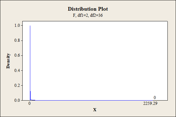
P-value for the main effect of A:
Software procedure:
Step-by-step procedure to find the P-value is given below:
- Click on Graph, select View Probability and click OK.
- Select F, enter 2 in numerator df and 36 in denominator df.
- Under Shaded Area Tab select X value under Define Shaded Area By and select right tails.
- Choose X value as 2,259.29.
- Click OK.
Output obtained from MINITAB is given below:
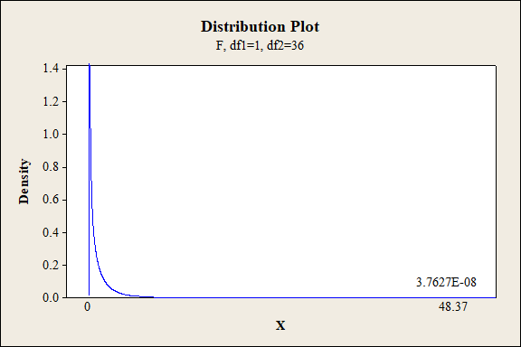
P-value for the main effect of B:
Software procedure:
Step-by-step procedure to find the P-value is given below:
- Click on Graph, select View Probability and click OK.
- Select F, enter 1 in numerator df and 36 in denominator df.
- Under Shaded Area Tab select X value under Define Shaded Area By and select right tails.
- Choose X value as 48.37.
- Click OK.
Output obtained from MINITAB is given below:
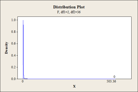
P-value for the main effect of C:
Software procedure:
Step-by-step procedure to find the P-value is given below:
- Click on Graph, select View Probability and click OK.
- Select F, enter 2 in numerator df and 36 in denominator df.
- Under Shaded Area Tab select X value under Define Shaded Area By and select right tails.
- Choose X value as 503.36.
- Click OK.
Output obtained from MINITAB is given below:
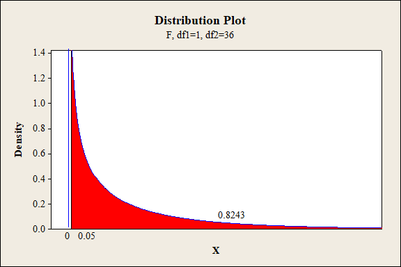
P-value for the main effect of D:
Software procedure:
Step-by-step procedure to find the P-value is given below:
- Click on Graph, select View Probability and click OK.
- Select F, enter 1 in numerator df and 36 in denominator df.
- Under Shaded Area Tab select X value under Define Shaded Area By and select right tails.
- Choose X value as 0.05.
- Click OK.
Output obtained from MINITAB is given below:
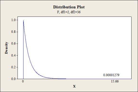
P-value for the interaction effect of A and B:
Software procedure:
Step-by-step procedure to find the P-value is given below:
- Click on Graph, select View Probability and click OK.
- Select F, enter 2 in numerator df and 36 in denominator df.
- Under Shaded Area Tab select X value under Define Shaded Area By and select right tails.
- Choose X value as 15.66.
- Click OK.
Output obtained from MINITAB is given below:
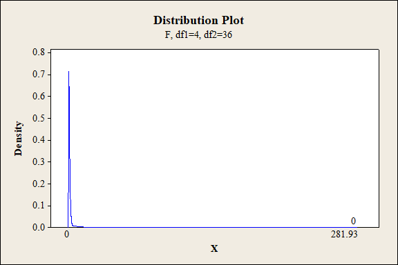
P-value for the interaction effect of A and C:
Software procedure:
Step-by-step procedure to find the P-value is given below:
- Click on Graph, select View Probability and click OK.
- Select F, enter 4 in numerator df and 36 in denominator df.
- Under Shaded Area Tab select X value under Define Shaded Area By and select right tails.
- Choose X value as 281.93.
- Click OK.
Output obtained from MINITAB is given below:
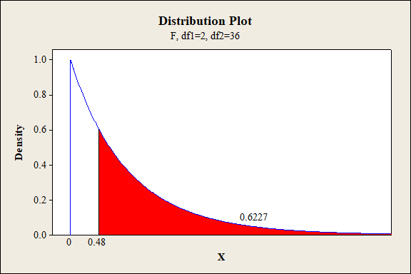
P-value for the interaction effect of A and D:
Software procedure:
Step-by-step procedure to find the P-value is given below:
- Click on Graph, select View Probability and click OK.
- Select F, enter 2 in numerator df and 36 in denominator df.
- Under Shaded Area Tab select X value under Define Shaded Area By and select right tails.
- Choose X value as 0.48.
- Click OK.
Output obtained from MINITAB is given below:
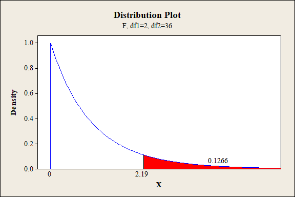
P-value for the interaction effect of B and C:
Software procedure:
Step-by-step procedure to find the P-value is given below:
- Click on Graph, select View Probability and click OK.
- Select F, enter 2 in numerator df and 36 in denominator df.
- Under Shaded Area Tab select X value under Define Shaded Area By and select right tails.
- Choose X value as 2.19.
- Click OK.
Output obtained from MINITAB is given below:
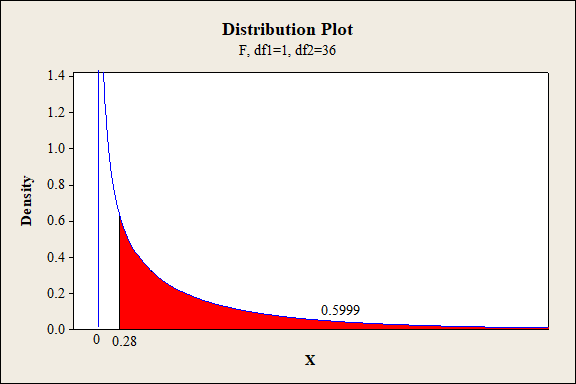
P-value for the interaction effect of B and D:
Software procedure:
Step-by-step procedure to find the P-value is given below:
- Click on Graph, select View Probability and click OK.
- Select F, enter 1 in numerator df and 36 in denominator df.
- Under Shaded Area Tab select X value under Define Shaded Area By and select right tails.
- Choose X value as 0.28.
- Click OK.
Output obtained from MINITAB is given below:
P-value for the interaction effect of C and D:
Software procedure:
Step-by-step procedure to find the P-value is given below:
- Click on Graph, select View Probability and click OK.
- Select F, enter 2 in numerator df and 36 in denominator df.
- Under Shaded Area Tab select X value under Define Shaded Area By and select right tails.
- Choose X value as 0.25.
- Click OK.
Output obtained from MINITAB is given below:

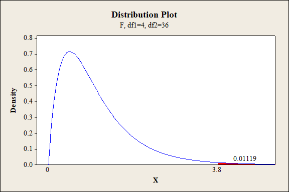
P-value for the interaction effect of A, B and C:
Software procedure:
Step-by-step procedure to find the P-value is given below:
- Click on Graph, select View Probability and click OK.
- Select F, enter 4 in numerator df and 36 in denominator df.
- Under Shaded Area Tab select X value under Define Shaded Area By and select right tails.
- Choose X value as 3.80.
- Click OK.
Output obtained from MINITAB is given below:
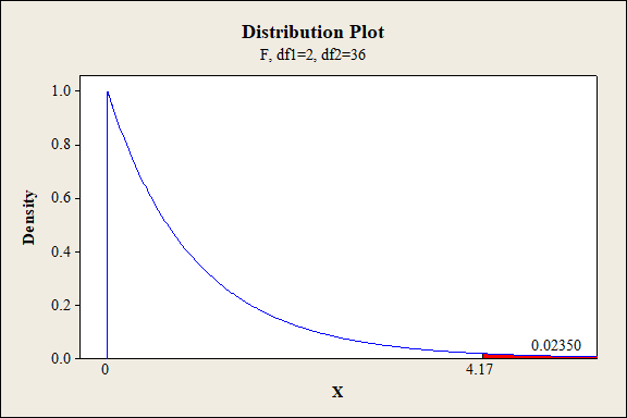
P-value for the interaction effect of A, B and D:
Software procedure:
Step-by-step procedure to find the P-value is given below:
- Click on Graph, select View Probability and click OK.
- Select F, enter 2 in numerator df and 36 in denominator df.
- Under Shaded Area Tab select X value under Define Shaded Area By and select right tails.
- Choose X value as 4.17.
- Click OK.
Output obtained from MINITAB is given below:
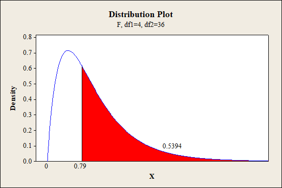
P-value for the interaction effect of A, C and D:
Software procedure:
Step-by-step procedure to find the P-value is given below:
- Click on Graph, select View Probability and click OK.
- Select F, enter 4 in numerator df and 36 in denominator df.
- Under Shaded Area Tab select X value under Define Shaded Area By and select right tails.
- Choose X value as 0.79.
- Click OK.
Output obtained from MINITAB is given below:
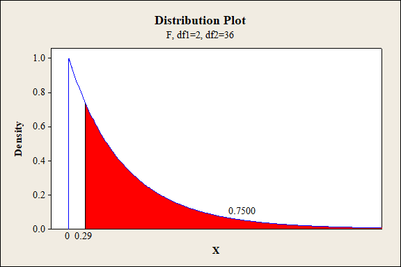
P-value for the interaction effect of B, C and D:
Software procedure:
Step-by-step procedure to find the P-value is given below:
- Click on Graph, select View Probability and click OK.
- Select F, enter 2 in numerator df and 36 in denominator df.
- Under Shaded Area Tab select X value under Define Shaded Area By and select right tails.
- Choose X value as 0.29.
- Click OK.
Output obtained from MINITAB is given below:
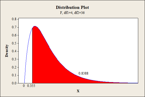
P-value for the interaction effect of A, B, C and D:
Software procedure:
Step-by-step procedure to find the P-value is given below:
- Click on Graph, select View Probability and click OK.
- Select F, enter 4 in numerator df and 36 in denominator df.
- Under Shaded Area Tab select X value under Define Shaded Area By and select right tails.
- Choose X value as 0.355.
- Click OK.
Output obtained from MINITAB is given below:
Conclusion:
For the main effect of A:
The P- value for the factor A (fabric) is 0.000 and the level of significance is 0.01.
Here, the P- value is lesser than the level of significance.
That is,
Thus, the null hypothesis is rejected,
Hence, there is sufficient of evidence to conclude that there is an effect of fabric on the extent of color change at 1% level of significance.
For main effect of B:
The P- value for the factor B (exposure level) is 0.000 and the level of significance is 0.01.
Here, the P- value is lesser than the level of significance.
That is,
Thus, the null hypothesis is not rejected.
Hence, there is sufficient of evidence to conclude that there is an effect exposure type on the extent of color change at 1% level of significance.
For main effect of C:
The P- value for the factor C (exposure level) is 0.000 and the level of significance is 0.01.
Here, the P- value is lesser than the level of significance.
That is,
Thus, the null hypothesis is rejected.
Hence, there is sufficient of evidence to conclude that there is an effect of exposure level on the extent of color change at 1% level of significance.
For main effect of D:
The P- value for the factor D (fabric direction) is 0.8243 and the level of significance is 0.01.
Here, the P- value is greater than the level of significance.
That is,
Thus, the null hypothesis is not rejected.
Hence, there is no sufficient of evidence to conclude that there is an effect of fabric direction on the extent of color change at 1% level of significance.
Interaction effect of factor A and B:
The P- value for the interaction effect AB (fabric and exposure type) is 0.000 and the level of significance is 0.01.
Here, the P- value is lesser than the level of significance.
That is,
Thus, the null hypothesis is rejected,
Hence, there is sufficient of evidence to conclude that there is an interaction effect of fabric and exposure type on the extent of color change at 1% level of significance.
Interaction effect of factor A and C:
The P- value for the interaction effect AC (fabric and exposure level) is 0.000 and the level of significance is 0.01.
Here, the P- value is lesser than the level of significance.
That is,
Thus, the null hypothesis is rejected.
Hence, there is sufficient of evidence to conclude that there is an interaction effect of fabric and exposure level on the extent of color change at 1% level of significance.
Interaction effect of factor A and D:
The P- value for the interaction effect AD (fabric and fabric direction) is 0.6227 and the level of significance is 0.01.
Here, the P- value is greater than the level of significance.
That is,
Thus, the null hypothesis is not rejected.
Hence, there is no sufficient of evidence to conclude that there is an interaction effect of fabric and fabric direction on the extent of color change at 1% level of significance.
Interaction effect of factor B and C:
The P- value for the interaction effect BC (exposure type and exposure level) is 0.1266 and the level of significance is 0.01.
Here, the P- value is greater than the level of significance.
That is,
Thus, the null hypothesis is not rejected,
Hence, there is no sufficient of evidence to conclude that there is an interaction effect of exposure type and exposure level on the extent of color change at 1% level of significance.
Interaction effect of factor B and D:
The P- value for the interaction effect BD (exposure type and fabric direction) is 0.5999 and the level of significance is 0.01.
Here, the P- value is greater than the level of significance.
That is,
Thus, the null hypothesis is not rejected,
Hence, there is no sufficient of evidence to conclude that there is an interaction effect of exposure type and fabric direction on the extent of color change at 1% level of significance.
Interaction effect of factor C and D:
The P- value for the interaction effect CD (exposure level and fabric direction) is 0.7801 and the level of significance is 0.01.
Here, the P- value is greater than the level of significance.
That is,
Thus, the null hypothesis is not rejected,
Hence, there is no sufficient of evidence to conclude that there is an interaction effect of exposure level and fabric direction on the extent of color change at 1% level of significance.
Interaction effect of factor A,B and C:
The P- value for the interaction effect ABC (fabric, exposure type and exposure level) is 0.01119 and the level of significance is 0.01.
Here, the P- value is greater than the level of significance.
That is,
Thus, the null hypothesis is not rejected.
Hence, there is no sufficient of evidence to conclude that there is an interaction effect of fabric, exposure type and exposure level on the extent of color change at 1% level of significance.
Interaction effect of factor A,B and D:
The P- value for the interaction effect ABD (fabric, exposure type and fabric direction) is 0.0235 and the level of significance is 0.01.
Here, the P- value is greater than the level of significance.
That is,
Thus, the null hypothesis is not rejected.
Hence, there is no sufficient of evidence to conclude that there is an interaction effect of fabric, exposure type and fabric direction on the extent of color change at 1% level of significance.
Interaction effect of factor A,C and D:
The P- value for the interaction effect ACD (fabric, exposure level and fabric direction) is 0.5394 and the level of significance is 0.01.
Here, the P- value is greater than the level of significance.
That is,
Thus, the null hypothesis is not rejected.
Hence, there is no sufficient of evidence to conclude that there is an interaction effect of fabric, exposure level and fabric direction on the extent of color change at 1% level of significance.
Interaction effect of factor B, C and D:
The P- value for the interaction effect BCD (exposure type, exposure level and fabric direction) is 0.7500 and the level of significance is 0.01.
Here, the P- value is greater than the level of significance.
That is,
Thus, the null hypothesis is not rejected.
Hence, there is no sufficient of evidence to conclude that there is an interaction effect of exposure type, exposure level and fabric direction on the extent of color change at 1% level of significance.
Interaction effect of factor A, B, C and D:
The P- value for the interaction effect ABCD (fabric, exposure type, exposure level and fabric direction) is 0.8388 and the level of significance is 0.01.
Here, the P- value is greater than the level of significance.
That is,
Thus, the null hypothesis is not rejected.
Hence, there is no sufficient of evidence to conclude that there is an interaction effect of fabric, exposure type, exposure level and fabric direction on the extent of color change at 1% level of significance.
Therefore, there is significant difference in the extent of color change with respect to the main effect A, B, D and interaction effects AB, AC are significant at 1% level of significance. The remaining second order interactions and third order interaction are not significant at 1% level of significance.
Want to see more full solutions like this?
Chapter 11 Solutions
Bundle: Probability and Statistics for Engineering and the Sciences, 9th + WebAssign Printed Access Card for Devore's Probability and Statistics for ... and the Sciences, 9th Edition, Single-Term


- 1. A consumer group claims that the mean annual consumption of cheddar cheese by a person in the United States is at most 10.3 pounds. A random sample of 100 people in the United States has a mean annual cheddar cheese consumption of 9.9 pounds. Assume the population standard deviation is 2.1 pounds. At a = 0.05, can you reject the claim? (Adapted from U.S. Department of Agriculture) State the hypotheses: Calculate the test statistic: Calculate the P-value: Conclusion (reject or fail to reject Ho): 2. The CEO of a manufacturing facility claims that the mean workday of the company's assembly line employees is less than 8.5 hours. A random sample of 25 of the company's assembly line employees has a mean workday of 8.2 hours. Assume the population standard deviation is 0.5 hour and the population is normally distributed. At a = 0.01, test the CEO's claim. State the hypotheses: Calculate the test statistic: Calculate the P-value: Conclusion (reject or fail to reject Ho): Statisticsarrow_forward21. find the mean. and variance of the following: Ⓒ x(t) = Ut +V, and V indepriv. s.t U.VN NL0, 63). X(t) = t² + Ut +V, U and V incepires have N (0,8) Ut ①xt = e UNN (0162) ~ X+ = UCOSTE, UNNL0, 62) SU, Oct ⑤Xt= 7 where U. Vindp.rus +> ½ have NL, 62). ⑥Xn = ΣY, 41, 42, 43, ... Yn vandom sample K=1 Text with mean zen and variance 6arrow_forwardA psychology researcher conducted a Chi-Square Test of Independence to examine whether there is a relationship between college students’ year in school (Freshman, Sophomore, Junior, Senior) and their preferred coping strategy for academic stress (Problem-Focused, Emotion-Focused, Avoidance). The test yielded the following result: image.png Interpret the results of this analysis. In your response, clearly explain: Whether the result is statistically significant and why. What this means about the relationship between year in school and coping strategy. What the researcher should conclude based on these findings.arrow_forward
- A school counselor is conducting a research study to examine whether there is a relationship between the number of times teenagers report vaping per week and their academic performance, measured by GPA. The counselor collects data from a sample of high school students. Write the null and alternative hypotheses for this study. Clearly state your hypotheses in terms of the correlation between vaping frequency and academic performance. EditViewInsertFormatToolsTable 12pt Paragrapharrow_forwardA smallish urn contains 25 small plastic bunnies – 7 of which are pink and 18 of which are white. 10 bunnies are drawn from the urn at random with replacement, and X is the number of pink bunnies that are drawn. (a) P(X = 5) ≈ (b) P(X<6) ≈ The Whoville small urn contains 100 marbles – 60 blue and 40 orange. The Grinch sneaks in one night and grabs a simple random sample (without replacement) of 15 marbles. (a) The probability that the Grinch gets exactly 6 blue marbles is [ Select ] ["≈ 0.054", "≈ 0.043", "≈ 0.061"] . (b) The probability that the Grinch gets at least 7 blue marbles is [ Select ] ["≈ 0.922", "≈ 0.905", "≈ 0.893"] . (c) The probability that the Grinch gets between 8 and 12 blue marbles (inclusive) is [ Select ] ["≈ 0.801", "≈ 0.760", "≈ 0.786"] . The Whoville small urn contains 100 marbles – 60 blue and 40 orange. The Grinch sneaks in one night and grabs a simple random sample (without replacement) of 15 marbles. (a)…arrow_forwardSuppose an experiment was conducted to compare the mileage(km) per litre obtained by competing brands of petrol I,II,III. Three new Mazda, three new Toyota and three new Nissan cars were available for experimentation. During the experiment the cars would operate under same conditions in order to eliminate the effect of external variables on the distance travelled per litre on the assigned brand of petrol. The data is given as below: Brands of Petrol Mazda Toyota Nissan I 10.6 12.0 11.0 II 9.0 15.0 12.0 III 12.0 17.4 13.0 (a) Test at the 5% level of significance whether there are signi cant differences among the brands of fuels and also among the cars. [10] (b) Compute the standard error for comparing any two fuel brands means. Hence compare, at the 5% level of significance, each of fuel brands II, and III with the standard fuel brand I. [10] �arrow_forward
- Analyze the residuals of a linear regression model and select the best response. yes, the residual plot does not show a curve no, the residual plot shows a curve yes, the residual plot shows a curve no, the residual plot does not show a curve I answered, "No, the residual plot shows a curve." (and this was incorrect). I am not sure why I keep getting these wrong when the answer seems obvious. Please help me understand what the yes and no references in the answer.arrow_forwarda. Find the value of A.b. Find pX(x) and py(y).c. Find pX|y(x|y) and py|X(y|x)d. Are x and y independent? Why or why not?arrow_forwardAnalyze the residuals of a linear regression model and select the best response.Criteria is simple evaluation of possible indications of an exponential model vs. linear model) no, the residual plot does not show a curve yes, the residual plot does not show a curve yes, the residual plot shows a curve no, the residual plot shows a curve I selected: yes, the residual plot shows a curve and it is INCORRECT. Can u help me understand why?arrow_forward
 Big Ideas Math A Bridge To Success Algebra 1: Stu...AlgebraISBN:9781680331141Author:HOUGHTON MIFFLIN HARCOURTPublisher:Houghton Mifflin Harcourt