Videos
Perform ANOVA to test the significance at 1% level of significance.
Answer to Problem 37E
The ANOVA for the given data is shown below:
| Source |
Degrees of freedom |
Sum of squares |
Mean sum of squares | F-ratio |
|
Fabric A | 2 | 4,414.658 | 2207.329 | 2259.293 |
|
Type of exposure B | 1 | 47.255 | 47.255 | 48.36745 |
|
Degree of exposure C | 2 | 983.566 | 491.783 | 503.3603 |
|
Fabric direction D | 1 | 0.044 | 0.044 | 0.045036 |
| Interaction AB | 2 | 30.606 | 15.303 | 15.66325 |
| Interaction AC | 2 | 1,101.754 | 275.446 | 281.9304 |
| Interaction AD | 2 | 0.94 | 0.47 | 0.481064 |
| Interaction BC | 2 | 4.282 | 2.141 | 2.191402 |
| Interaction BD | 1 | 0.273 | 0.273 | 0.279427 |
| Interaction CD | 2 | 0.494 | 0.247 | 0.252815 |
| Interaction ABC | 4 | 14.856 | 3.714 | 3.801433 |
| Interaction ABD | 2 | 8.144 | 4.072 | 4.167861 |
|
Interaction ACD | 4 | 3.068 | 0.767 | 0.785056 |
|
Interaction BCD | 2 | 0.56 | 0.28 | 0.286592 |
| Interaction ABCD | 4 | 1.389 | 0.347 | 0.355 |
| Error | 36 | 35.172 | 0.977 | |
| Total | 71 | 6,647.091 | 9.621 |
There is sufficient of evidence to conclude that there is an effect of fabric on the extent of color change at 1% level of significance.
There is sufficient of evidence to conclude that there is an effect exposure type on the extent of color change at 1% level of significance.
There is sufficient of evidence to conclude that there is an effect of exposure level on the extent of color change at 1% level of significance.
There is no sufficient of evidence to conclude that there is an effect of fabric direction on the extent of color change at 1% level of significance.
There is sufficient of evidence to conclude that there is an interaction effect of fabric and exposure type on the extent of color change at 1% level of significance.
There is sufficient of evidence to conclude that there is an interaction effect of fabric and exposure level on the extent of color change at 1% level of significance.
There is no sufficient of evidence to conclude that there is an interaction effect of fabric and fabric direction on the extent of color change at 1% level of significance.
There is no sufficient of evidence to conclude that there is an interaction effect of exposure type and exposure level on the extent of color change at 1% level of significance.
There is no sufficient of evidence to conclude that there is an interaction effect of exposure type and fabric direction on the extent of color change at 1% level of significance.
There is no sufficient of evidence to conclude that there is an interaction effect of exposure level and fabric direction on the extent of color change at 1% level of significance.
There is no sufficient of evidence to conclude that there is an interaction effect of fabric, exposure type and exposure level on the extent of color change at 1% level of significance.
There is no sufficient of evidence to conclude that there is an interaction effect of fabric, exposure type and fabric direction on the extent of color change at 1% level of significance.
There is no sufficient of evidence to conclude that there is an interaction effect of fabric, exposure level and fabric direction on the extent of color change at 1% level of significance.
There is no sufficient of evidence to conclude that there is an interaction effect of exposure type, exposure level and fabric direction on the extent of color change at 1% level of significance.
There is no sufficient of evidence to conclude that there is an interaction effect of fabric, exposure type, exposure level and fabric direction on the extent of color change at 1% level of significance.
Explanation of Solution
Given info:
An experiment was conducted to test the effect of fabric, type of exposure, level of exposure and fabric direction on the color change of the fabric. Two observation were noted for each of the four factors.
Calculation:
The general ANOVA table is given below:
| Source | Degrees of freedom | Sum of squares | Mean sum of squares | F-ratio |
| Factor A | ||||
| Factor B | ||||
| Factor C | ||||
| Factor D | ||||
| Interaction AB | ||||
| Interaction ABC | ||||
| Error | ||||
| Total |
The sum of squares for each factor and interaction is calculated by multiplying the mean sum of squares with its corresponding degrees of freedom.
Sum of squares excluding ABCD:
| Source | Sum of squares |
| A | 4,414.658 |
| B | 47.255 |
| C | 983.566 |
| D | 0.044 |
| AB | 30.606 |
| AC | 1,101.784 |
| AD | 0.94 |
| BC | 4.282 |
| BD | 0.273 |
| CD | 0.494 |
| ABC | 14.856 |
| ABD | 8.144 |
| ACD | 3.068 |
| BCD | 0.56 |
| Error | 35.172 |
| Total | 6,647.091 |
Using the above table SSABCD can be calculated:
The mean sum of squares for the interaction ABCD is given below:
Thus, the mean sum of squares for the interaction ABCD is 0.347.
The ANOVA for the given data is shown below:
| Source | Degrees of freedom |
Sum of squares |
Mean sum of squares | F-ratio |
|
Fabric A | 4,414.658 | 2207.329 | 2,259.293 | |
|
Type of exposure B | 47.255 | 47.255 | 48.36745 | |
|
Degree of exposure C | 983.566 | 491.783 | 503.3603 | |
|
Fabric direction D | 0.044 | 0.044 | 0.045036 | |
|
Interaction AB | 30.606 | 15.303 | 15.66325 | |
|
Interaction AC | 1,101.754 | 275.446 | 281.9304 | |
|
Interaction AD | 0.94 | 0.47 | 0.481064 | |
|
Interaction BC | 4.282 | 2.141 | 2.191402 | |
|
Interaction BD | 0.273 | 0.273 | 0.279427 | |
|
Interaction CD | 0.494 | 0.247 | 0.252815 | |
|
Interaction ABC | 14.856 | 3.714 | 3.801433 | |
|
Interaction ABD | 8.144 | 4.072 | 4.167861 | |
|
Interaction ACD | 3.068 | 0.767 | 0.785056 | |
|
Interaction BCD | 0.56 | 0.28 | 0.286592 | |
|
Interaction ABCD | 1.389 | 0.347 | 0.355 | |
| Error | 35.172 | 0.977 | ||
| Total | 6,647.091 | 9.621 |
Where,
The F statistic for each factor is obtained by dividing the mean sum of squares with the mean sum of squares due to error.
Testing the main effects:
Testing the Hypothesis for the factor A:
Null hypothesis:
That is, there is no significant difference in the extent of color change due to the three levels of fabrics.
Alternative hypothesis:
That is, there is significant difference in the extent of color change due to the three levels of fabrics.
Testing the Hypothesis for the factor B:
Null hypothesis:
That is, there is no significant difference in the extent of color change due to the two levels of exposure type.
Alternative hypothesis:
That is, there is a significant difference in the extent of color change due to the two levels of exposure type.
Testing the Hypothesis for the factor C:
Null hypothesis:
That is, there is no significant difference in the extent of color change due to the three levels of exposure level.
Alternative hypothesis:
That is, there is a significant difference in the extent of color change due to the three levels of exposure level.
Testing the Hypothesis for the factor D:
Null hypothesis:
That is, there is no significant difference in the extent of color change due to the two levels of fabric direction.
Alternative hypothesis:
That is, there is a significant difference in the extent of color change due to the two levels of fabric direction.
Testing the Hypothesis for the interaction effect of AB:
Null hypothesis:
That is, there is no significant difference in the extent of color change due to the interaction between fabric and exposure type.
Alternative hypothesis:
That is, there is significant difference in the extent of color change due to the interaction between fabric and exposure type.
Testing the Hypothesis for the interaction effect AC:
Null hypothesis:
That is, there is no significant difference in the extent of color change due to the interaction between fabric and exposure level.
Alternative hypothesis:
That is, there is a significant difference in the extent of color change due to the interaction between fabric and exposure level.
Testing the Hypothesis for the interaction effect AD:
Null hypothesis:
That is, there is no significant difference in the extent of color change due to the interaction between fabric and fabric direction.
Alternative hypothesis:
That is, there is a significant difference in the extent of color change due to the interaction between fabric and fabric direction.
Testing the Hypothesis for the interaction effect BC:
Null hypothesis:
That is, there is no significant difference in the extent of color change due to the interaction between exposure type and exposure level.
Alternative hypothesis:
That is, there is significant difference in the extent of color change due to the interaction between exposure type and exposure level.
Testing the Hypothesis for the interaction effect BD:
Null hypothesis:
That is, there is no significant difference in the extent of color change due to the interaction between exposure type and fabric direction.
Alternative hypothesis:
That is, there is significant difference in the extent of color change due to the interaction between exposure type and fabric direction.
Testing the Hypothesis for the interaction effect CD:
Null hypothesis:
That is, there is no significant difference in the extent of color change due to the interaction between exposure level and fabric direction.
Alternative hypothesis:
That is, there is significant difference in the extent of color change due to the interaction between exposure level and fabric direction.
Testing the Hypothesis for the interaction effect ABC:
Null hypothesis:
That is, there is no significant difference in the extent of color change due to the interaction between fabric, exposure type and exposure level.
Alternative hypothesis:
That is, there is a significant difference in the extent of color change due to the interaction between fabric, exposure type and exposure level.
Testing the Hypothesis for the interaction effect ABD:
Null hypothesis:
That is, there is no significant difference in the extent of color change due to the interaction between fabric, exposure type and fabric direction.
Alternative hypothesis:
That is, there is a significant difference in the extent of color change due to the interaction between fabric, exposure type and fabric direction.
Testing the Hypothesis for the interaction effect ACD:
Null hypothesis:
That is, there is no significant difference in the extent of color change due to the interaction between fabric, exposure level and fabric direction.
Alternative hypothesis:
That is, there is a significant difference in the extent of color change due to the interaction between fabric, exposure level and fabric direction.
Testing the Hypothesis for the interaction effect BCD:
Null hypothesis:
That is, there is no significant difference in the extent of color change due to the interaction between exposure type, exposure level and fabric direction.
Alternative hypothesis:
That is, there is a significant difference in the extent of color change due to the interaction between exposure type, exposure level and fabric direction.
Testing the Hypothesis for the interaction effect ABCD:
Null hypothesis:
That is, there is no significant difference in the extent of color change due to the interaction between exposure type, exposure level and fabric direction.
Alternative hypothesis:
That is, there is a significant difference in the extent of color change due to the interaction between fabric, exposure type, exposure level and fabric direction.
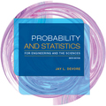
P-value for the main effect of A:
Software procedure:
Step-by-step procedure to find the P-value is given below:
- Click on Graph, select View Probability and click OK.
- Select F, enter 2 in numerator df and 36 in denominator df.
- Under Shaded Area Tab select X value under Define Shaded Area By and select right tails.
- Choose X value as 2,259.29.
- Click OK.
Output obtained from MINITAB is given below:
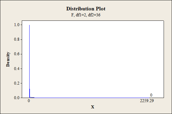
P-value for the main effect of B:
Software procedure:
Step-by-step procedure to find the P-value is given below:
- Click on Graph, select View Probability and click OK.
- Select F, enter 1 in numerator df and 36 in denominator df.
- Under Shaded Area Tab select X value under Define Shaded Area By and select right tails.
- Choose X value as 48.37.
- Click OK.
Output obtained from MINITAB is given below:
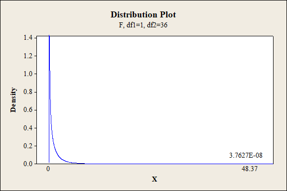
P-value for the main effect of C:
Software procedure:
Step-by-step procedure to find the P-value is given below:
- Click on Graph, select View Probability and click OK.
- Select F, enter 2 in numerator df and 36 in denominator df.
- Under Shaded Area Tab select X value under Define Shaded Area By and select right tails.
- Choose X value as 503.36.
- Click OK.
Output obtained from MINITAB is given below:
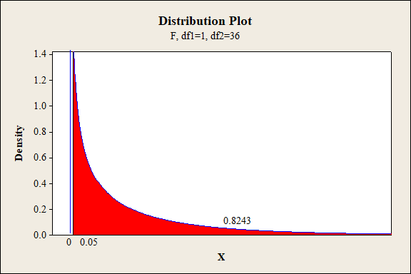
P-value for the main effect of D:
Software procedure:
Step-by-step procedure to find the P-value is given below:
- Click on Graph, select View Probability and click OK.
- Select F, enter 1 in numerator df and 36 in denominator df.
- Under Shaded Area Tab select X value under Define Shaded Area By and select right tails.
- Choose X value as 0.05.
- Click OK.
Output obtained from MINITAB is given below:
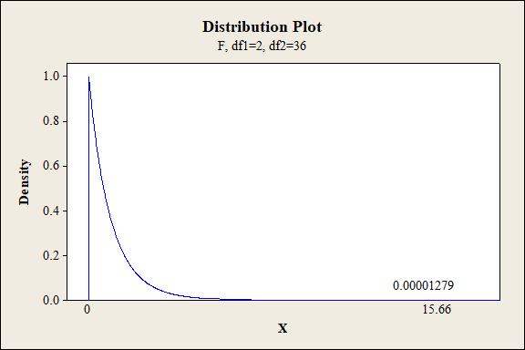
P-value for the interaction effect of A and B:
Software procedure:
Step-by-step procedure to find the P-value is given below:
- Click on Graph, select View Probability and click OK.
- Select F, enter 2 in numerator df and 36 in denominator df.
- Under Shaded Area Tab select X value under Define Shaded Area By and select right tails.
- Choose X value as 15.66.
- Click OK.
Output obtained from MINITAB is given below:
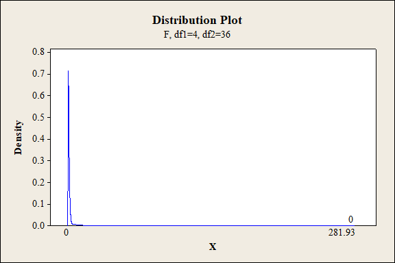
P-value for the interaction effect of A and C:
Software procedure:
Step-by-step procedure to find the P-value is given below:
- Click on Graph, select View Probability and click OK.
- Select F, enter 4 in numerator df and 36 in denominator df.
- Under Shaded Area Tab select X value under Define Shaded Area By and select right tails.
- Choose X value as 281.93.
- Click OK.
Output obtained from MINITAB is given below:
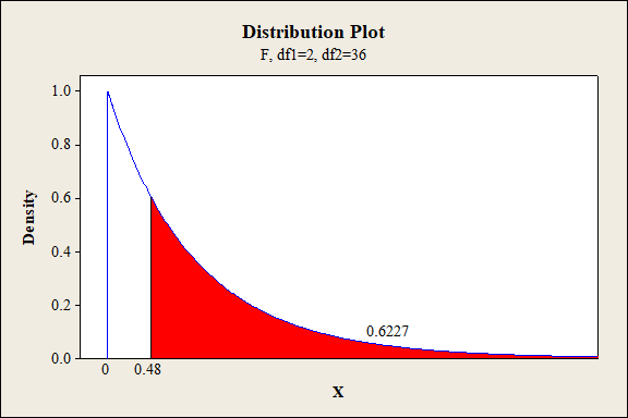
P-value for the interaction effect of A and D:
Software procedure:
Step-by-step procedure to find the P-value is given below:
- Click on Graph, select View Probability and click OK.
- Select F, enter 2 in numerator df and 36 in denominator df.
- Under Shaded Area Tab select X value under Define Shaded Area By and select right tails.
- Choose X value as 0.48.
- Click OK.
Output obtained from MINITAB is given below:
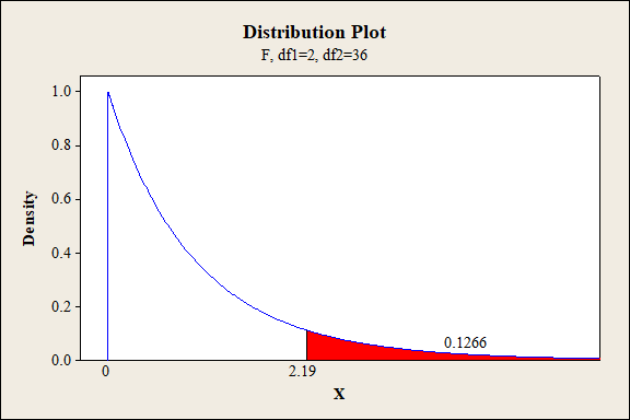
P-value for the interaction effect of B and C:
Software procedure:
Step-by-step procedure to find the P-value is given below:
- Click on Graph, select View Probability and click OK.
- Select F, enter 2 in numerator df and 36 in denominator df.
- Under Shaded Area Tab select X value under Define Shaded Area By and select right tails.
- Choose X value as 2.19.
- Click OK.
Output obtained from MINITAB is given below:
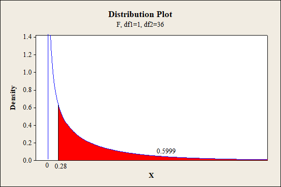
P-value for the interaction effect of B and D:
Software procedure:
Step-by-step procedure to find the P-value is given below:
- Click on Graph, select View Probability and click OK.
- Select F, enter 1 in numerator df and 36 in denominator df.
- Under Shaded Area Tab select X value under Define Shaded Area By and select right tails.
- Choose X value as 0.28.
- Click OK.
Output obtained from MINITAB is given below:
P-value for the interaction effect of C and D:
Software procedure:
Step-by-step procedure to find the P-value is given below:
- Click on Graph, select View Probability and click OK.
- Select F, enter 2 in numerator df and 36 in denominator df.
- Under Shaded Area Tab select X value under Define Shaded Area By and select right tails.
- Choose X value as 0.25.
- Click OK.
Output obtained from MINITAB is given below:

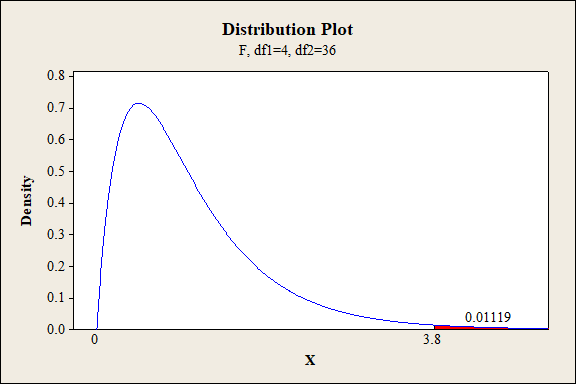
P-value for the interaction effect of A, B and C:
Software procedure:
Step-by-step procedure to find the P-value is given below:
- Click on Graph, select View Probability and click OK.
- Select F, enter 4 in numerator df and 36 in denominator df.
- Under Shaded Area Tab select X value under Define Shaded Area By and select right tails.
- Choose X value as 3.80.
- Click OK.
Output obtained from MINITAB is given below:
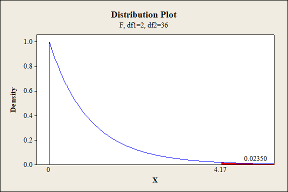
P-value for the interaction effect of A, B and D:
Software procedure:
Step-by-step procedure to find the P-value is given below:
- Click on Graph, select View Probability and click OK.
- Select F, enter 2 in numerator df and 36 in denominator df.
- Under Shaded Area Tab select X value under Define Shaded Area By and select right tails.
- Choose X value as 4.17.
- Click OK.
Output obtained from MINITAB is given below:
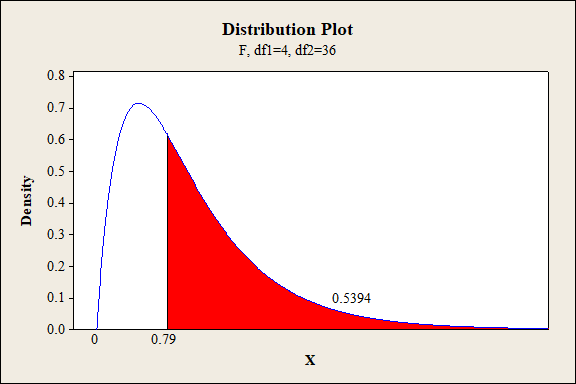
P-value for the interaction effect of A, C and D:
Software procedure:
Step-by-step procedure to find the P-value is given below:
- Click on Graph, select View Probability and click OK.
- Select F, enter 4 in numerator df and 36 in denominator df.
- Under Shaded Area Tab select X value under Define Shaded Area By and select right tails.
- Choose X value as 0.79.
- Click OK.
Output obtained from MINITAB is given below:
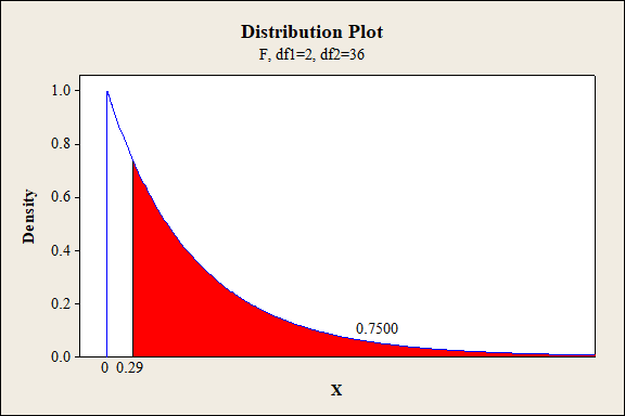
P-value for the interaction effect of B, C and D:
Software procedure:
Step-by-step procedure to find the P-value is given below:
- Click on Graph, select View Probability and click OK.
- Select F, enter 2 in numerator df and 36 in denominator df.
- Under Shaded Area Tab select X value under Define Shaded Area By and select right tails.
- Choose X value as 0.29.
- Click OK.
Output obtained from MINITAB is given below:
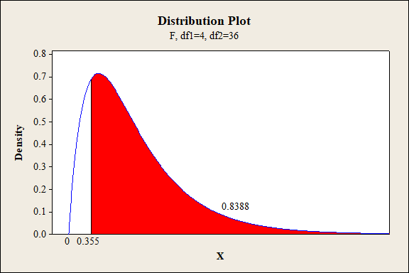
P-value for the interaction effect of A, B, C and D:
Software procedure:
Step-by-step procedure to find the P-value is given below:
- Click on Graph, select View Probability and click OK.
- Select F, enter 4 in numerator df and 36 in denominator df.
- Under Shaded Area Tab select X value under Define Shaded Area By and select right tails.
- Choose X value as 0.355.
- Click OK.
Output obtained from MINITAB is given below:
Conclusion:
For the main effect of A:
The P- value for the factor A (fabric) is 0.000 and the level of significance is 0.01.
Here, the P- value is lesser than the level of significance.
That is,
Thus, the null hypothesis is rejected,
Hence, there is sufficient of evidence to conclude that there is an effect of fabric on the extent of color change at 1% level of significance.
For main effect of B:
The P- value for the factor B (exposure level) is 0.000 and the level of significance is 0.01.
Here, the P- value is lesser than the level of significance.
That is,
Thus, the null hypothesis is not rejected.
Hence, there is sufficient of evidence to conclude that there is an effect exposure type on the extent of color change at 1% level of significance.
For main effect of C:
The P- value for the factor C (exposure level) is 0.000 and the level of significance is 0.01.
Here, the P- value is lesser than the level of significance.
That is,
Thus, the null hypothesis is rejected.
Hence, there is sufficient of evidence to conclude that there is an effect of exposure level on the extent of color change at 1% level of significance.
For main effect of D:
The P- value for the factor D (fabric direction) is 0.8243 and the level of significance is 0.01.
Here, the P- value is greater than the level of significance.
That is,
Thus, the null hypothesis is not rejected.
Hence, there is no sufficient of evidence to conclude that there is an effect of fabric direction on the extent of color change at 1% level of significance.
Interaction effect of factor A and B:
The P- value for the interaction effect AB (fabric and exposure type) is 0.000 and the level of significance is 0.01.
Here, the P- value is lesser than the level of significance.
That is,
Thus, the null hypothesis is rejected,
Hence, there is sufficient of evidence to conclude that there is an interaction effect of fabric and exposure type on the extent of color change at 1% level of significance.
Interaction effect of factor A and C:
The P- value for the interaction effect AC (fabric and exposure level) is 0.000 and the level of significance is 0.01.
Here, the P- value is lesser than the level of significance.
That is,
Thus, the null hypothesis is rejected.
Hence, there is sufficient of evidence to conclude that there is an interaction effect of fabric and exposure level on the extent of color change at 1% level of significance.
Interaction effect of factor A and D:
The P- value for the interaction effect AD (fabric and fabric direction) is 0.6227 and the level of significance is 0.01.
Here, the P- value is greater than the level of significance.
That is,
Thus, the null hypothesis is not rejected.
Hence, there is no sufficient of evidence to conclude that there is an interaction effect of fabric and fabric direction on the extent of color change at 1% level of significance.
Interaction effect of factor B and C:
The P- value for the interaction effect BC (exposure type and exposure level) is 0.1266 and the level of significance is 0.01.
Here, the P- value is greater than the level of significance.
That is,
Thus, the null hypothesis is not rejected,
Hence, there is no sufficient of evidence to conclude that there is an interaction effect of exposure type and exposure level on the extent of color change at 1% level of significance.
Interaction effect of factor B and D:
The P- value for the interaction effect BD (exposure type and fabric direction) is 0.5999 and the level of significance is 0.01.
Here, the P- value is greater than the level of significance.
That is,
Thus, the null hypothesis is not rejected,
Hence, there is no sufficient of evidence to conclude that there is an interaction effect of exposure type and fabric direction on the extent of color change at 1% level of significance.
Interaction effect of factor C and D:
The P- value for the interaction effect CD (exposure level and fabric direction) is 0.7801 and the level of significance is 0.01.
Here, the P- value is greater than the level of significance.
That is,
Thus, the null hypothesis is not rejected,
Hence, there is no sufficient of evidence to conclude that there is an interaction effect of exposure level and fabric direction on the extent of color change at 1% level of significance.
Interaction effect of factor A,B and C:
The P- value for the interaction effect ABC (fabric, exposure type and exposure level) is 0.01119 and the level of significance is 0.01.
Here, the P- value is greater than the level of significance.
That is,
Thus, the null hypothesis is not rejected.
Hence, there is no sufficient of evidence to conclude that there is an interaction effect of fabric, exposure type and exposure level on the extent of color change at 1% level of significance.
Interaction effect of factor A,B and D:
The P- value for the interaction effect ABD (fabric, exposure type and fabric direction) is 0.0235 and the level of significance is 0.01.
Here, the P- value is greater than the level of significance.
That is,
Thus, the null hypothesis is not rejected.
Hence, there is no sufficient of evidence to conclude that there is an interaction effect of fabric, exposure type and fabric direction on the extent of color change at 1% level of significance.
Interaction effect of factor A,C and D:
The P- value for the interaction effect ACD (fabric, exposure level and fabric direction) is 0.5394 and the level of significance is 0.01.
Here, the P- value is greater than the level of significance.
That is,
Thus, the null hypothesis is not rejected.
Hence, there is no sufficient of evidence to conclude that there is an interaction effect of fabric, exposure level and fabric direction on the extent of color change at 1% level of significance.
Interaction effect of factor B, C and D:
The P- value for the interaction effect BCD (exposure type, exposure level and fabric direction) is 0.7500 and the level of significance is 0.01.
Here, the P- value is greater than the level of significance.
That is,
Thus, the null hypothesis is not rejected.
Hence, there is no sufficient of evidence to conclude that there is an interaction effect of exposure type, exposure level and fabric direction on the extent of color change at 1% level of significance.
Interaction effect of factor A, B, C and D:
The P- value for the interaction effect ABCD (fabric, exposure type, exposure level and fabric direction) is 0.8388 and the level of significance is 0.01.
Here, the P- value is greater than the level of significance.
That is,
Thus, the null hypothesis is not rejected.
Hence, there is no sufficient of evidence to conclude that there is an interaction effect of fabric, exposure type, exposure level and fabric direction on the extent of color change at 1% level of significance.
Therefore, there is significant difference in the extent of color change with respect to the main effect A, B, D and interaction effects AB, AC are significant at 1% level of significance. The remaining second order interactions and third order interaction are not significant at 1% level of significance.
Want to see more full solutions like this?
Chapter 11 Solutions
EBK PROBABILITY AND STATISTICS FOR ENGI


- Show that L′(θ) = Cθ394(1 −2θ)604(395 −2000θ).arrow_forwarda) Let X and Y be independent random variables both with the same mean µ=0. Define a new random variable W = aX +bY, where a and b are constants. (i) Obtain an expression for E(W).arrow_forwardThe table below shows the estimated effects for a logistic regression model with squamous cell esophageal cancer (Y = 1, yes; Y = 0, no) as the response. Smoking status (S) equals 1 for at least one pack per day and 0 otherwise, alcohol consumption (A) equals the average number of alcohoic drinks consumed per day, and race (R) equals 1 for blacks and 0 for whites. Variable Effect (β) P-value Intercept -7.00 <0.01 Alcohol use 0.10 0.03 Smoking 1.20 <0.01 Race 0.30 0.02 Race × smoking 0.20 0.04 Write-out the prediction equation (i.e., the logistic regression model) when R = 0 and again when R = 1. Find the fitted Y S conditional odds ratio in each case. Next, write-out the logistic regression model when S = 0 and again when S = 1. Find the fitted Y R conditional odds ratio in each case.arrow_forward
- The chi-squared goodness-of-fit test can be used to test if data comes from a specific continuous distribution by binning the data to make it categorical. Using the OpenIntro Statistics county_complete dataset, test the hypothesis that the persons_per_household 2019 values come from a normal distribution with mean and standard deviation equal to that variable's mean and standard deviation. Use signficance level a = 0.01. In your solution you should 1. Formulate the hypotheses 2. Fill in this table Range (-⁰⁰, 2.34] (2.34, 2.81] (2.81, 3.27] (3.27,00) Observed 802 Expected 854.2 The first row has been filled in. That should give you a hint for how to calculate the expected frequencies. Remember that the expected frequencies are calculated under the assumption that the null hypothesis is true. FYI, the bounderies for each range were obtained using JASP's drag-and-drop cut function with 8 levels. Then some of the groups were merged. 3. Check any conditions required by the chi-squared…arrow_forwardSuppose that you want to estimate the mean monthly gross income of all households in your local community. You decide to estimate this population parameter by calling 150 randomly selected residents and asking each individual to report the household’s monthly income. Assume that you use the local phone directory as the frame in selecting the households to be included in your sample. What are some possible sources of error that might arise in your effort to estimate the population mean?arrow_forwardFor the distribution shown, match the letter to the measure of central tendency. A B C C Drag each of the letters into the appropriate measure of central tendency. Mean C Median A Mode Barrow_forward
- A physician who has a group of 38 female patients aged 18 to 24 on a special diet wishes to estimate the effect of the diet on total serum cholesterol. For this group, their average serum cholesterol is 188.4 (measured in mg/100mL). Suppose that the total serum cholesterol measurements are normally distributed with standard deviation of 40.7. (a) Find a 95% confidence interval of the mean serum cholesterol of patients on the special diet.arrow_forwardThe accompanying data represent the weights (in grams) of a simple random sample of 10 M&M plain candies. Determine the shape of the distribution of weights of M&Ms by drawing a frequency histogram. Find the mean and median. Which measure of central tendency better describes the weight of a plain M&M? Click the icon to view the candy weight data. Draw a frequency histogram. Choose the correct graph below. ○ A. ○ C. Frequency Weight of Plain M and Ms 0.78 0.84 Frequency OONAG 0.78 B. 0.9 0.96 Weight (grams) Weight of Plain M and Ms 0.84 0.9 0.96 Weight (grams) ○ D. Candy Weights 0.85 0.79 0.85 0.89 0.94 0.86 0.91 0.86 0.87 0.87 - Frequency ☑ Frequency 67200 0.78 → Weight of Plain M and Ms 0.9 0.96 0.84 Weight (grams) Weight of Plain M and Ms 0.78 0.84 Weight (grams) 0.9 0.96 →arrow_forwardThe acidity or alkalinity of a solution is measured using pH. A pH less than 7 is acidic; a pH greater than 7 is alkaline. The accompanying data represent the pH in samples of bottled water and tap water. Complete parts (a) and (b). Click the icon to view the data table. (a) Determine the mean, median, and mode pH for each type of water. Comment on the differences between the two water types. Select the correct choice below and fill in any answer boxes in your choice. A. For tap water, the mean pH is (Round to three decimal places as needed.) B. The mean does not exist. Data table Тар 7.64 7.45 7.45 7.10 7.46 7.50 7.68 7.69 7.56 7.46 7.52 7.46 5.15 5.09 5.31 5.20 4.78 5.23 Bottled 5.52 5.31 5.13 5.31 5.21 5.24 - ☑arrow_forward
- く Chapter 5-Section 1 Homework X MindTap - Cengage Learning x + C webassign.net/web/Student/Assignment-Responses/submit?pos=3&dep=36701632&tags=autosave #question3874894_3 M Gmail 品 YouTube Maps 5. [-/20 Points] DETAILS MY NOTES BBUNDERSTAT12 5.1.020. ☆ B Verify it's you Finish update: All Bookmarks PRACTICE ANOTHER A computer repair shop has two work centers. The first center examines the computer to see what is wrong, and the second center repairs the computer. Let x₁ and x2 be random variables representing the lengths of time in minutes to examine a computer (✗₁) and to repair a computer (x2). Assume x and x, are independent random variables. Long-term history has shown the following times. 01 Examine computer, x₁₁ = 29.6 minutes; σ₁ = 8.1 minutes Repair computer, X2: μ₂ = 92.5 minutes; σ2 = 14.5 minutes (a) Let W = x₁ + x2 be a random variable representing the total time to examine and repair the computer. Compute the mean, variance, and standard deviation of W. (Round your answers…arrow_forwardThe acidity or alkalinity of a solution is measured using pH. A pH less than 7 is acidic; a pH greater than 7 is alkaline. The accompanying data represent the pH in samples of bottled water and tap water. Complete parts (a) and (b). Click the icon to view the data table. (a) Determine the mean, median, and mode pH for each type of water. Comment on the differences between the two water types. Select the correct choice below and fill in any answer boxes in your choice. A. For tap water, the mean pH is (Round to three decimal places as needed.) B. The mean does not exist. Data table Тар Bottled 7.64 7.45 7.46 7.50 7.68 7.45 7.10 7.56 7.46 7.52 5.15 5.09 5.31 5.20 4.78 5.52 5.31 5.13 5.31 5.21 7.69 7.46 5.23 5.24 Print Done - ☑arrow_forwardThe median for the given set of six ordered data values is 29.5. 9 12 23 41 49 What is the missing value? The missing value is ☐.arrow_forward
 Big Ideas Math A Bridge To Success Algebra 1: Stu...AlgebraISBN:9781680331141Author:HOUGHTON MIFFLIN HARCOURTPublisher:Houghton Mifflin Harcourt