
INTRODUCTORY STAT. W/MYLAB MATH>CUSTOM<
3rd Edition
ISBN: 9780135231548
Author: Gould
Publisher: PEARSON C
expand_more
expand_more
format_list_bulleted
Videos
Textbook Question
Chapter 11, Problem 50SE
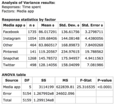
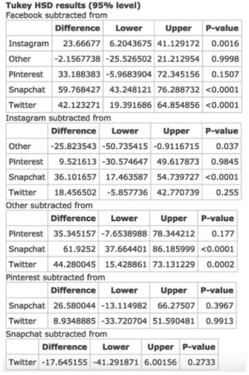
Social Media Use A StatCrunch survey asked respondents how much time they spent daily on various social media sites. Is there a difference in the
Expert Solution & Answer
Want to see the full answer?
Check out a sample textbook solution
Students have asked these similar questions
Business discuss
Spam filters are built on principles similar to those used in logistic regression. We fit a probability that each message is spam or not spam. We have several variables for each email. Here are a few: to_multiple=1 if there are multiple recipients, winner=1 if the word 'winner' appears in the subject line, format=1 if the email is poorly formatted, re_subj=1 if "re" appears in the subject line. A logistic model was fit to a dataset with the following output:
Estimate
SE
Z
Pr(>|Z|)
(Intercept)
-0.8161
0.086
-9.4895
0
to_multiple
-2.5651
0.3052
-8.4047
0
winner
1.5801
0.3156
5.0067
0
format
-0.1528
0.1136
-1.3451
0.1786
re_subj
-2.8401
0.363
-7.824
0
(a) Write down the model using the coefficients from the model fit.log_odds(spam) = -0.8161 + -2.5651 + to_multiple + 1.5801 winner + -0.1528 format + -2.8401 re_subj(b) Suppose we have an observation where to_multiple=0, winner=1, format=0, and re_subj=0. What is the predicted probability that this message is spam?…
Consider an event X comprised of three outcomes whose probabilities are 9/18, 1/18,and 6/18.
Compute the probability of the complement of the event.
Question content area bottom
Part 1
A.1/2
B.2/18
C.16/18
D.16/3
Chapter 11 Solutions
INTRODUCTORY STAT. W/MYLAB MATH>CUSTOM<
Ch. 11 - In Exercises 11.1 and 11.2, for each situation,...Ch. 11 - In Exercises 11.1 and 11.2, for each situation,...Ch. 11 - Bonferroni Correction (Example 1) Suppose you have...Ch. 11 - Prob. 4SECh. 11 - Apartment Rents Random samples of rents for...Ch. 11 - Prob. 6SECh. 11 - Gas Prices The website Gasbuddy.com reports the...Ch. 11 - More Gas Prices The following table shows the...Ch. 11 - Prob. 9SECh. 11 - Prob. 10SE
Ch. 11 - Gas Price Intervals Use the data from exercise...Ch. 11 - Gas Price Intervals Use the data from exercise...Ch. 11 - Prob. 13SECh. 11 - Baseball Position and Hits Use the data in the...Ch. 11 - Comparing F -Values from Boxplots (Example 3)...Ch. 11 - Comparing F -Values from Boxplots Refer to the...Ch. 11 - Marital Status and Cholesterol (Example 4) Refer...Ch. 11 - Marital Status and Blood Pressure Test the...Ch. 11 - Schoolwork and Class (Example 5) A random survey...Ch. 11 - TV Hours A random survey was done at a small...Ch. 11 - Schoolwork and Class Use the information for...Ch. 11 - TV Hours Use the information for exercise 11.20....Ch. 11 - Schoolwork Again Go back to the information in...Ch. 11 - TV Hours Again Go back to the information in...Ch. 11 - Pulse Rates (Example 6) Pulse rates were taken for...Ch. 11 - UCLA Music Survey The figure shows side-by-side...Ch. 11 - Commute Times by Method A survey was given to...Ch. 11 - Gas Price ANOVA Based on the following output,...Ch. 11 - Apartment Rents (Example 7) Samples of rents for...Ch. 11 - Study Hours by Major Three independent random...Ch. 11 - Salary by Type of College Information was gathered...Ch. 11 - Draft Lottery When the draft lottery for military...Ch. 11 - Reaction Times for Athletes A random sample of...Ch. 11 - Tomato Plants and Colored Light Jennifer Brogan, a...Ch. 11 - GPAs by Seating Choice A random sample of students...Ch. 11 - Reading Comprehension Sixty-six reading students...Ch. 11 - Hours of Steep and Health Status In a study done...Ch. 11 - Happiness and Age Category StatCrunch surveyed...Ch. 11 - Prob. 41SECh. 11 - House Prices Tukey HSD confidence intervals (with...Ch. 11 - GPA and Row (Example 8) A random sample of...Ch. 11 - Reading Scores by Teaching Method Refer to...Ch. 11 - Reaction Distances Use the data given in exercise...Ch. 11 - Study Hours Use the data given in exercise 11.32....Ch. 11 - Prob. 47SECh. 11 - Tomatoes Use the data given in exercise 11.36....Ch. 11 - Concern over Nuclear Power Following the...Ch. 11 - Social Media Use A StatCrunch survey asked...Ch. 11 - Happiness and Age Consider the data from the...Ch. 11 - GPA and Row Number Suppose you collect data on...Ch. 11 - Contacting Mother Professors of ethics (Eth),...Ch. 11 - Ideal Percentage to Charity Professors of ethics...Ch. 11 - Actual Percentage to Charity Professors of ethics...Ch. 11 - Hours of Television by Age Group The StatCrunch...Ch. 11 - Triglycerides and Gender Using the NHANES data, we...Ch. 11 - Cholesterol and Gender Using NHANES data, we...
Knowledge Booster


Learn more about
Need a deep-dive on the concept behind this application? Look no further. Learn more about this topic, statistics and related others by exploring similar questions and additional content below.Similar questions
- John and Mike were offered mints. What is the probability that at least John or Mike would respond favorably? (Hint: Use the classical definition.) Question content area bottom Part 1 A.1/2 B.3/4 C.1/8 D.3/8arrow_forwardThe details of the clock sales at a supermarket for the past 6 weeks are shown in the table below. The time series appears to be relatively stable, without trend, seasonal, or cyclical effects. The simple moving average value of k is set at 2. What is the simple moving average root mean square error? Round to two decimal places. Week Units sold 1 88 2 44 3 54 4 65 5 72 6 85 Question content area bottom Part 1 A. 207.13 B. 20.12 C. 14.39 D. 0.21arrow_forwardThe details of the clock sales at a supermarket for the past 6 weeks are shown in the table below. The time series appears to be relatively stable, without trend, seasonal, or cyclical effects. The simple moving average value of k is set at 2. If the smoothing constant is assumed to be 0.7, and setting F1 and F2=A1, what is the exponential smoothing sales forecast for week 7? Round to the nearest whole number. Week Units sold 1 88 2 44 3 54 4 65 5 72 6 85 Question content area bottom Part 1 A. 80 clocks B. 60 clocks C. 70 clocks D. 50 clocksarrow_forward
- The details of the clock sales at a supermarket for the past 6 weeks are shown in the table below. The time series appears to be relatively stable, without trend, seasonal, or cyclical effects. The simple moving average value of k is set at 2. Calculate the value of the simple moving average mean absolute percentage error. Round to two decimal places. Week Units sold 1 88 2 44 3 54 4 65 5 72 6 85 Part 1 A. 14.39 B. 25.56 C. 23.45 D. 20.90arrow_forwardThe accompanying data shows the fossil fuels production, fossil fuels consumption, and total energy consumption in quadrillions of BTUs of a certain region for the years 1986 to 2015. Complete parts a and b. Year Fossil Fuels Production Fossil Fuels Consumption Total Energy Consumption1949 28.748 29.002 31.9821950 32.563 31.632 34.6161951 35.792 34.008 36.9741952 34.977 33.800 36.7481953 35.349 34.826 37.6641954 33.764 33.877 36.6391955 37.364 37.410 40.2081956 39.771 38.888 41.7541957 40.133 38.926 41.7871958 37.216 38.717 41.6451959 39.045 40.550 43.4661960 39.869 42.137 45.0861961 40.307 42.758 45.7381962 41.732 44.681 47.8261963 44.037 46.509 49.6441964 45.789 48.543 51.8151965 47.235 50.577 54.0151966 50.035 53.514 57.0141967 52.597 55.127 58.9051968 54.306 58.502 62.4151969 56.286…arrow_forwardThe accompanying data shows the fossil fuels production, fossil fuels consumption, and total energy consumption in quadrillions of BTUs of a certain region for the years 1986 to 2015. Complete parts a and b. Year Fossil Fuels Production Fossil Fuels Consumption Total Energy Consumption1949 28.748 29.002 31.9821950 32.563 31.632 34.6161951 35.792 34.008 36.9741952 34.977 33.800 36.7481953 35.349 34.826 37.6641954 33.764 33.877 36.6391955 37.364 37.410 40.2081956 39.771 38.888 41.7541957 40.133 38.926 41.7871958 37.216 38.717 41.6451959 39.045 40.550 43.4661960 39.869 42.137 45.0861961 40.307 42.758 45.7381962 41.732 44.681 47.8261963 44.037 46.509 49.6441964 45.789 48.543 51.8151965 47.235 50.577 54.0151966 50.035 53.514 57.0141967 52.597 55.127 58.9051968 54.306 58.502 62.4151969 56.286…arrow_forward
- The accompanying data shows the fossil fuels production, fossil fuels consumption, and total energy consumption in quadrillions of BTUs of a certain region for the years 1986 to 2015. Complete parts a and b. Develop line charts for each variable and identify the characteristics of the time series (that is, random, stationary, trend, seasonal, or cyclical). What is the line chart for the variable Fossil Fuels Production?arrow_forwardThe accompanying data shows the fossil fuels production, fossil fuels consumption, and total energy consumption in quadrillions of BTUs of a certain region for the years 1986 to 2015. Complete parts a and b. Year Fossil Fuels Production Fossil Fuels Consumption Total Energy Consumption1949 28.748 29.002 31.9821950 32.563 31.632 34.6161951 35.792 34.008 36.9741952 34.977 33.800 36.7481953 35.349 34.826 37.6641954 33.764 33.877 36.6391955 37.364 37.410 40.2081956 39.771 38.888 41.7541957 40.133 38.926 41.7871958 37.216 38.717 41.6451959 39.045 40.550 43.4661960 39.869 42.137 45.0861961 40.307 42.758 45.7381962 41.732 44.681 47.8261963 44.037 46.509 49.6441964 45.789 48.543 51.8151965 47.235 50.577 54.0151966 50.035 53.514 57.0141967 52.597 55.127 58.9051968 54.306 58.502 62.4151969 56.286…arrow_forwardFor each of the time series, construct a line chart of the data and identify the characteristics of the time series (that is, random, stationary, trend, seasonal, or cyclical). Month PercentApr 1972 4.97May 1972 5.00Jun 1972 5.04Jul 1972 5.25Aug 1972 5.27Sep 1972 5.50Oct 1972 5.73Nov 1972 5.75Dec 1972 5.79Jan 1973 6.00Feb 1973 6.02Mar 1973 6.30Apr 1973 6.61May 1973 7.01Jun 1973 7.49Jul 1973 8.30Aug 1973 9.23Sep 1973 9.86Oct 1973 9.94Nov 1973 9.75Dec 1973 9.75Jan 1974 9.73Feb 1974 9.21Mar 1974 8.85Apr 1974 10.02May 1974 11.25Jun 1974 11.54Jul 1974 11.97Aug 1974 12.00Sep 1974 12.00Oct 1974 11.68Nov 1974 10.83Dec 1974 10.50Jan 1975 10.05Feb 1975 8.96Mar 1975 7.93Apr 1975 7.50May 1975 7.40Jun 1975 7.07Jul 1975 7.15Aug 1975 7.66Sep 1975 7.88Oct 1975 7.96Nov 1975 7.53Dec 1975 7.26Jan 1976 7.00Feb 1976 6.75Mar 1976 6.75Apr 1976 6.75May 1976…arrow_forward
- Hi, I need to make sure I have drafted a thorough analysis, so please answer the following questions. Based on the data in the attached image, develop a regression model to forecast the average sales of football magazines for each of the seven home games in the upcoming season (Year 10). That is, you should construct a single regression model and use it to estimate the average demand for the seven home games in Year 10. In addition to the variables provided, you may create new variables based on these variables or based on observations of your analysis. Be sure to provide a thorough analysis of your final model (residual diagnostics) and provide assessments of its accuracy. What insights are available based on your regression model?arrow_forwardI want to make sure that I included all possible variables and observations. There is a considerable amount of data in the images below, but not all of it may be useful for your purposes. Are there variables contained in the file that you would exclude from a forecast model to determine football magazine sales in Year 10? If so, why? Are there particular observations of football magazine sales from previous years that you would exclude from your forecasting model? If so, why?arrow_forwardStat questionsarrow_forward
arrow_back_ios
SEE MORE QUESTIONS
arrow_forward_ios
Recommended textbooks for you
 Glencoe Algebra 1, Student Edition, 9780079039897...AlgebraISBN:9780079039897Author:CarterPublisher:McGraw Hill
 College Algebra (MindTap Course List)AlgebraISBN:9781305652231Author:R. David Gustafson, Jeff HughesPublisher:Cengage Learning
Glencoe Algebra 1, Student Edition, 9780079039897...
Algebra
ISBN:9780079039897
Author:Carter
Publisher:McGraw Hill
College Algebra (MindTap Course List)
Algebra
ISBN:9781305652231
Author:R. David Gustafson, Jeff Hughes
Publisher:Cengage Learning
Hypothesis Testing using Confidence Interval Approach; Author: BUM2413 Applied Statistics UMP;https://www.youtube.com/watch?v=Hq1l3e9pLyY;License: Standard YouTube License, CC-BY
Hypothesis Testing - Difference of Two Means - Student's -Distribution & Normal Distribution; Author: The Organic Chemistry Tutor;https://www.youtube.com/watch?v=UcZwyzwWU7o;License: Standard Youtube License