Concept explainers
Videos
(a)
To find: The distribution of present and past year total billing and total number of architects, staff, and engineers by using numerical and graphical summaries.
(a)
Answer to Problem 26E
Solution: The distribution of present and past year total billing and total number of architects and engineers is positively skewed. The distribution of staff has some missing frequencies but it can be said that it is approximately skewed to right.
Explanation of Solution
Calculation: To show the distribution of present and past year total billing and total number of architects, staff, and engineers, create the histogram. To obtain the histogram by using Minitab, follow the steps below:
Step 1: Open the Minitab worksheet which contains the data.
Step 2: Go to Graph > Histogram Boxplot > Simple.
Step 3: Click OK.
Step 4: Select “ArchBill13, ArchBill12 N_Arch, N_En, and N_Staff” in the column for Graph variables.
Step 5: Go to multiple graphs “In separate panels of the same graph.”
Step 6: Click “OK.” Again click “OK.”
A histogram with the numerical summaries is obtained. The obtained histogram is shown below:
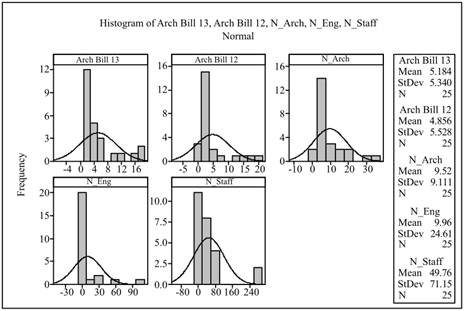
Interpretation: It can be seen from the obtained histogram that the distribution of present and past year total billing and total number of architects and engineers is positively skewed. It means the data are skewed to right. The distribution of staff has some missing frequencies but it can be said that it is approximately skewed to right.
(b)
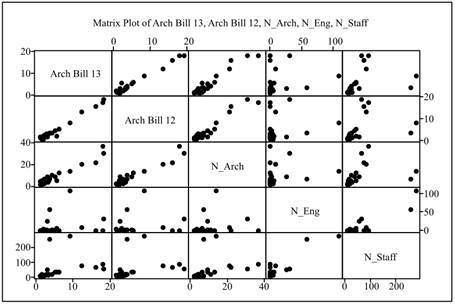
To find: The relationship for every variable by using numerical and graphical summaries.
(b)
Answer to Problem 26E
Solution: There is a
Explanation of Solution
Calculation: To show the relationship between the present and past year total billing and total number of architects, staff, and engineers, obtain the
Step 1: Open the Minitab worksheet which contains the data.
Step 2: Go to Graph> Matrix plot> Simple > OK.
Step 3: Select “ArchBill13, ArchBill12 N_Arch, N_En, and N_Staff” in the column for Graph Variables.
Step 4: Click “OK.”
The scatterplot is obtained for all the variables. Obtained scatterplot is shown below:
To show the relationship between the present and past year total billing and total number of architects, staff and engineers, obtain the
Step 1: Open the Minitab worksheet which contains the data.
Step 2: Go to Stat> Stat> Basic statistics > Correlation.
Step 3: Select “ArchBill13, ArchBill12 N_Arch, N_En, and N_Staff” in the column for Variables.
Step 4: Click “OK.”
The correlation between present year and total number of architects is obtained as 0.962. The correlation between present year and total number of staff is obtained as 0.373. The correlation between present year and total number of engineers is obtained as 0.230. The correlation between past year and total number of engineers is obtained as 0.204. The correlation between past year and total number of staff is obtained as 0.349. The correlation between past year and total number of architects is obtained as 0.959.
Interpretation: The correlation between present year and total number of architects is obtained as 0.962 and the correlation between past year and total number of architects is obtained as 0.959. It indicates that there is a positive correlation between the variables. The value of correlation is near to 1, hence it can be concluded that the variables present year and total number of architects and the variables past year and total number of architects are strong and positively correlated. The correlation between present year and total number of staff is obtained as 0.373, the correlation between present year and total number of engineers is obtained as 0.230, the correlation between past year and total number of engineers is obtained as 0.204, and the correlation between past year and total number of staff is obtained as 0.349. It indicates that there is a positive correlation between the variables. The value of correlation is small, hence it can be concluded that the variables are not strong but positively correlated. The scatterplot plot also represents the similar results.
(c)
To test: A multiple regression with the fitted equation.
(c)
Answer to Problem 26E
Solution: A regression model of present year and total number of architects, staff, and engineers is
Explanation of Solution
Calculation: To perform the multiple regression by using year and census count as explanatory variables use Minitab and follow the steps given below:
Step 1: Open the Minitab worksheet which contains the data.
Step 2: Go to Stat> Regression > Regression > Fit regression model.
Step 3: Select ArchBill13 in the column for Response and select N_Arch, N_En, and N_Staff in the column for Predictors.
Step 4: Click “OK.”
Step 5: Again go to Stat> Regression > Regression > Fit regression model.
Step 6: Select ArchBill12 in the column for Response and select N_Arch, N_En, and N_Staff in the column for Predictors.
Step 7: Click “OK.”
Conclusion: A regression model of present year and total number of architects, staff, and engineers is
(d)
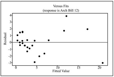
To find: The residuals.
(d)
Answer to Problem 26E
Solution: The table representing the residuals is shown below:
Residuals for past year |
Residuals for present year |
1.93465 |
1.03345 |
3.86630 |
4.04527 |
1.73284 |
0.64784 |
0.30066 |
0.41724 |
2.40798 |
|
0.26357 |
0.36849 |
0.33508 |
0.39052 |
1.49413 |
1.20884 |
1.58345 |
0.88167 |
1.47193 |
0.66624 |
0.55973 |
|
0.21479 |
|
0.27727 |
0.65183 |
0.00292 |
|
1.06694 |
0.34126 |
The data points are randomly scattered and does not represent any pattern.
Explanation of Solution
Calculation: To obtain the residuals by using Minitab, follow the steps below:
Step 1: Open the Minitab worksheet that contains the data.
Step 2: Go to Stat> Regression > General regression.
Step 3: Select ArchBill12 in the column for Response and select N_Arch, N_En, and N_Staff in the column for Predictors.
Step 4: Click on storage and select “Residuals.” Click on Graphs and select “Residuals versus fits.”
Step 5: Again go to Stat> Regression > General regression.
Step 6: Select ArchBill13 in the column for Response and select N_Arch, N_En, and N_Staff in the column for Predictors.
Step 7: Click on storage and select “Residuals.” Click on Graphs and select “Residuals versus fits.”
Step 8: Click “OK.”
The residuals and the residual plot are obtained. The table representing the residuals is shown below:
Residuals for past year |
Residuals for present year |
1.93465 |
1.03345 |
3.86630 |
4.04527 |
1.73284 |
0.64784 |
0.30066 |
0.41724 |
2.40798 |
|
0.26357 |
0.36849 |
0.33508 |
0.39052 |
1.49413 |
1.20884 |
1.58345 |
0.88167 |
1.47193 |
0.66624 |
0.55973 |
|
0.21479 |
|
0.27727 |
0.65183 |
0.00292 |
|
1.06694 |
0.34126 |
The obtained residual plot for the past year is shown below:
The obtained residual plot for the present year is shown below:
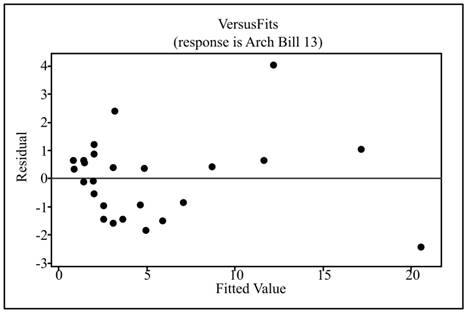
Interpretation: From the obtained residual plots, it can be seen that the data points are randomly scattered and does not represent any pattern.
(e)
To find: The predicted total billing for the previous year.
(e)
Answer to Problem 26E
Solution: The predicted total billing for the previous year is 1.028.
Explanation of Solution
Calculation: The predicted total billing for the provided data can be obtained by using Minitab. Steps are as follows:
Step 1: Open the Minitab worksheet which contains the data.
Step 2: Go to Stat> Regression > General regression.
Step 3: Select ArchBill12 in the column for Response and select N_Arch, N_En, and N_Staff in the column for Predictors.
Step 4: Click on Options and write 3, 1 and 17 in the column for Prediction intervals for new observations.
Step 5: Click “OK.”
The predicted value is obtained as 1.028.
(f)
To explain: The use of statistical inference under this setting.
(f)
Answer to Problem 26E
Solution: The use of statistical inference under this setting did not justify the data as data does not follow
Explanation of Solution
Step 1: Open the Minitab worksheet that contains the data.
Step 2: Go to Graph > Probability Plot > Single > Click OK.
Step 3: Select ArchBill12, ArchBill13, N_Arch, N_En, and N_Staff in the column for Graph variables.
The obtained Normal quantile plot is shown below:
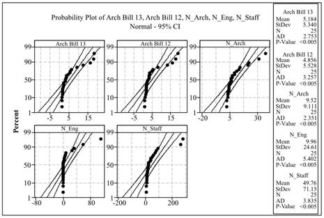
From the obtained normal quantile plot, it can be seen that the residuals deviate from the line. So, it can be concluded that the data does not follow normal distribution. From the part (a), it can be seen that all the variables are skewed to right.
In the provided problem, it can be seen that all the variables are positively correlated. The variables are correlated and randomly distributed. The data are skewed to right. From the normal quantile plot, it can be seen that the residuals deviate from the line. So, it can be concluded that the data does not follow normal distributed.
Want to see more full solutions like this?
Chapter 11 Solutions
EBK INTRODUCTION TO THE PRACTICE OF STA


- What would you say about a set of quantitative bivariate data whose linear correlation is -1? What would a scatter diagram of the data look like? (5 points)arrow_forwardBusiness discussarrow_forwardAnalyze the residuals of a linear regression model and select the best response. yes, the residual plot does not show a curve no, the residual plot shows a curve yes, the residual plot shows a curve no, the residual plot does not show a curve I answered, "No, the residual plot shows a curve." (and this was incorrect). I am not sure why I keep getting these wrong when the answer seems obvious. Please help me understand what the yes and no references in the answer.arrow_forward
- a. Find the value of A.b. Find pX(x) and py(y).c. Find pX|y(x|y) and py|X(y|x)d. Are x and y independent? Why or why not?arrow_forwardAnalyze the residuals of a linear regression model and select the best response.Criteria is simple evaluation of possible indications of an exponential model vs. linear model) no, the residual plot does not show a curve yes, the residual plot does not show a curve yes, the residual plot shows a curve no, the residual plot shows a curve I selected: yes, the residual plot shows a curve and it is INCORRECT. Can u help me understand why?arrow_forwardYou have been hired as an intern to run analyses on the data and report the results back to Sarah; the five questions that Sarah needs you to address are given below. please do it step by step on excel Does there appear to be a positive or negative relationship between price and screen size? Use a scatter plot to examine the relationship. Determine and interpret the correlation coefficient between the two variables. In your interpretation, discuss the direction of the relationship (positive, negative, or zero relationship). Also discuss the strength of the relationship. Estimate the relationship between screen size and price using a simple linear regression model and interpret the estimated coefficients. (In your interpretation, tell the dollar amount by which price will change for each unit of increase in screen size). Include the manufacturer dummy variable (Samsung=1, 0 otherwise) and estimate the relationship between screen size, price and manufacturer dummy as a multiple…arrow_forward
- Here is data with as the response variable. x y54.4 19.124.9 99.334.5 9.476.6 0.359.4 4.554.4 0.139.2 56.354 15.773.8 9-156.1 319.2Make a scatter plot of this data. Which point is an outlier? Enter as an ordered pair, e.g., (x,y). (x,y)= Find the regression equation for the data set without the outlier. Enter the equation of the form mx+b rounded to three decimal places. y_wo= Find the regression equation for the data set with the outlier. Enter the equation of the form mx+b rounded to three decimal places. y_w=arrow_forwardYou have been hired as an intern to run analyses on the data and report the results back to Sarah; the five questions that Sarah needs you to address are given below. please do it step by step Does there appear to be a positive or negative relationship between price and screen size? Use a scatter plot to examine the relationship. Determine and interpret the correlation coefficient between the two variables. In your interpretation, discuss the direction of the relationship (positive, negative, or zero relationship). Also discuss the strength of the relationship. Estimate the relationship between screen size and price using a simple linear regression model and interpret the estimated coefficients. (In your interpretation, tell the dollar amount by which price will change for each unit of increase in screen size). Include the manufacturer dummy variable (Samsung=1, 0 otherwise) and estimate the relationship between screen size, price and manufacturer dummy as a multiple linear…arrow_forwardExercises: Find all the whole number solutions of the congruence equation. 1. 3x 8 mod 11 2. 2x+3= 8 mod 12 3. 3x+12= 7 mod 10 4. 4x+6= 5 mod 8 5. 5x+3= 8 mod 12arrow_forward
- Scenario Sales of products by color follow a peculiar, but predictable, pattern that determines how many units will sell in any given year. This pattern is shown below Product Color 1995 1996 1997 Red 28 42 21 1998 23 1999 29 2000 2001 2002 Unit Sales 2003 2004 15 8 4 2 1 2005 2006 discontinued Green 26 39 20 22 28 14 7 4 2 White 43 65 33 36 45 23 12 Brown 58 87 44 48 60 Yellow 37 56 28 31 Black 28 42 21 Orange 19 29 Purple Total 28 42 21 49 68 78 95 123 176 181 164 127 24 179 Questions A) Which color will sell the most units in 2007? B) Which color will sell the most units combined in the 2007 to 2009 period? Please show all your analysis, leave formulas in cells, and specify any assumptions you make.arrow_forwardOne hundred students were surveyed about their preference between dogs and cats. The following two-way table displays data for the sample of students who responded to the survey. Preference Male Female TOTAL Prefers dogs \[36\] \[20\] \[56\] Prefers cats \[10\] \[26\] \[36\] No preference \[2\] \[6\] \[8\] TOTAL \[48\] \[52\] \[100\] problem 1 Find the probability that a randomly selected student prefers dogs.Enter your answer as a fraction or decimal. \[P\left(\text{prefers dogs}\right)=\] Incorrect Check Hide explanation Preference Male Female TOTAL Prefers dogs \[\blueD{36}\] \[\blueD{20}\] \[\blueE{56}\] Prefers cats \[10\] \[26\] \[36\] No preference \[2\] \[6\] \[8\] TOTAL \[48\] \[52\] \[100\] There were \[\blueE{56}\] students in the sample who preferred dogs out of \[100\] total students.arrow_forwardBusiness discussarrow_forward
 MATLAB: An Introduction with ApplicationsStatisticsISBN:9781119256830Author:Amos GilatPublisher:John Wiley & Sons Inc
 Probability and Statistics for Engineering and th...StatisticsISBN:9781305251809Author:Jay L. DevorePublisher:Cengage Learning
 Statistics for The Behavioral Sciences (MindTap C...StatisticsISBN:9781305504912Author:Frederick J Gravetter, Larry B. WallnauPublisher:Cengage Learning
 Elementary Statistics: Picturing the World (7th E...StatisticsISBN:9780134683416Author:Ron Larson, Betsy FarberPublisher:PEARSON
 The Basic Practice of StatisticsStatisticsISBN:9781319042578Author:David S. Moore, William I. Notz, Michael A. FlignerPublisher:W. H. Freeman
 Introduction to the Practice of StatisticsStatisticsISBN:9781319013387Author:David S. Moore, George P. McCabe, Bruce A. CraigPublisher:W. H. Freeman