Chapter 11, Problem 21E

(a)

To determine

To find: The multiple regression for BMI using $x_1\text{and }{x}_2$ as explanatory variables.

Answer to Problem 21E

Solution: The required multiple regression model is $\underset{\_}{\text{BMI}=23.4-0.682x_1+0.102x_2}$.

Explanation of Solution

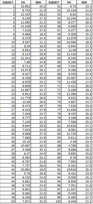
Given: The data for the PA and BMI are given below:

Calculation: The explanatory variables are $x_1=\left(\text{PA}-8.614\right){\text{and x}}_2={\left(\text{PA}-8.614\right)}^2$

To obtain multiple regression analysis by using Minitab, follow the steps below:

Step 1: Enter the data in Minitab worksheet.

Step 2: Go to Calc>Calculator.

Step 3: Enter $x_1=PA-8.614$ in Store result in variable for Expression.

Step 4: Click OK.

Step 5: Repeat the steps. Enter $x_2={\left(\text{PA}-8.614\right)}^2$ in Store result in variable for Expression.

Step 6: Go to Stat > Regression > Regression

Step 7: Select BMI in Response and select $x_1\text{ and }{x}_2$ in Predictors.

Step 8: Click OK.

The multiple regression model is obtained as $\text{BMI}=23.4-0.682x_1+0.102x_2$.

(b)

To determine

To find: The value of $R^2$.

Answer to Problem 21E

Solution: The value of $R^2$ 17.7%.

Explanation of Solution

It can be seen from part (b) that $R^2$ is obtained as 17.7% which is explained by predictors $x_1\text{ and }{x}_2$. The percentage of $R^2$ is very low. It indicates that the model is not good with this quadratic term.

(c)

To determine

To graph: The Normal quantile plot.

Explanation of Solution

Graph: To perform the multiple regression by using year and census count as explanatory variables use Minitab. Follow the steps below:

Step 1: Enter the data in Minitab worksheet.

Step 2: Go to Stat> Regression >Regression.

Step 3: Select BMI in Response and select $x_1\text{ and }{x}_2$ in Predictors.

Step 4: Click on Graphs and select “Residuals versus fits.”

Step 5: Click OK.

The residual plot is obtained as:

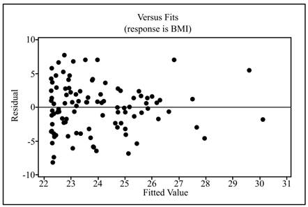
Interpretation: From the obtained residual plot, it can be concluded that the plot represents no pattern and the data points are randomly scattered.

(d)

To determine

To test: The hypothesis that coefficient of the variable $\text{PA}-8.614$ is equal to zero.

Answer to Problem 21E

Solution: There is enough evidence to conclude that there is no linear increase over time.

Explanation of Solution

Calculation: From the output which is obtained in part (b), the regression equation is $\text{BMI}=23.4-0.682x_1+0.102x_2$. The standard error is 0.0555. From the equation, it can be seen that the coefficient of $x_2\text{ is }{b}_2=0.102$. To test the hypothesis that there is a linear rise over time, the null and alternative hypotheses can be stated as:

$\begin{array}{l}{H}_0:{\beta }_2=0\\ H_{\alpha }:{\beta }_2\ne 0\end{array}$

The level of significance is 0.05. The test statistic under null hypothesis is calculated as:

$\begin{array}{c}t=\frac{b_2}{s_{b_1}}\\ =\frac{0.102}{0.05556}\\ =1.835\end{array}$

The p-value can be calculated as:

$\begin{array}{c}p-value=2P\left(t\ge \left|t_{cal}\right|\right)\\ =2P\left(t\ge 1.835\right)\\ =2\left(0.034\right)\\ =0.0678\end{array}$

The p-value is 0.0678.

Conclusion: The obtained p-value is greater than the significance level. Hence, there is enough evidence to conclude that the quadratic term contributes insignificantly to the fit.