Chapter 11, Problem 20E

(a)

To determine

The percentage of the overall population for each age group for the year 1950 and 2050.

Answer to Problem 20E

Solution: The percentage of the overall population for each age group for the year 1950 and 2050 are obtained as follows:

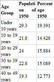
Age Group	Population of 1950	Percentage 1950	Population of 2050	Percentage 2050
Under 10 years	29.3	19.3911	56.2	18.0940
10 to 19 years	21.8	14.4275	56.7	18.2550
20 to 29 years	24.0	15.8835	56.2	18.0940
30 to 39 years	22.8	15.0893	55.9	17.9974
40 to 49 years	19.3	12.7730	52.8	16.9994
50 to 59 years	15.5	10.2581	49.1	15.8081
60 to 69 years	11.0	7.2799	45.0	14.4881
70 to 79 years	5.5	3.6400	34.5	11.1075
80 to 89 years	1.6	1.0589	23.7	7.6304
90 to 99 years	0.1	0.0662	8.1	2.6079
100 years and over			0.6	0.1932

Explanation of Solution

Calculation:

The percentage of the total population can be obtained by using the formula

$\text{Percentage}=\frac{\text{Population in an age group}}{\text{Total population}}\times 100$

The percentage of the total population can be calculated by using the Minitab software. The below steps are followed to obtained the required percentage for each age group for both the years.

Step 1: Enter the population for both the year 1950 and 2050.

Step 2: Go to Calc $\to$ Calculator and input the name of the column in “Store result in the variable.”

Step 3: Enter the required expression in the “Expression” column and click on OK.

Step 4: Repeat the process for both the years.

The obtained result is shown in the below table:

Age Group	Population of 1950	Percentage 1950	Population of 2050	Percentage 2050
Under 10 years	29.3	19.3911	56.2	18.0940
10 to 19 years	21.8	14.4275	56.7	18.2550
20 to 29 years	24.0	15.8835	56.2	18.0940
30 to 39 years	22.8	15.0893	55.9	17.9974
40 to 49 years	19.3	12.7730	52.8	16.9994
50 to 59 years	15.5	10.2581	49.1	15.8081
60 to 69 years	11.0	7.2799	45.0	14.4881
70 to 79 years	5.5	3.6400	34.5	11.1075
80 to 89 years	1.6	1.0589	23.7	7.6304
90 to 99 years	0.1	0.0662	8.1	2.6079
100 years and over			0.6	0.1932

(b)

To determine

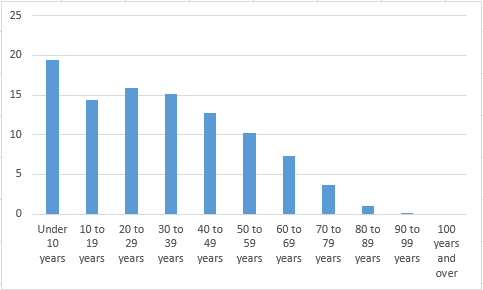
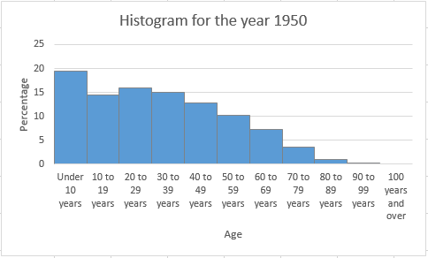
To graph: The histogram for the percentage of the population of the year 1950.

Explanation of Solution

Graph: To obtain the histogram for the obtained result in previous part, Excel is used. The below steps are followed to obtain the required histogram.

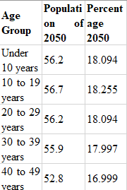
Step 1: The data is entered in the Excel worksheet. The snapshot of the obtained table is shown below:

Step 2: Select the data set and go to insert and select the option of cluster column under the Recommended Charts. The screenshot is shown below:

Step 3: Click on OK. The diagram is obtained as follows:

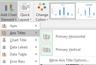
Step 4: Click on the chart area and select the option of “Primary Horizontal” and “Primary Vertical” axis under the “Add Chart Element” to add the axis title. The screenshot is shown below:

Step 5: Click on the bars of the diagrams and reduce the gap width to zero under the “Format Data Series” tab. The screenshot is shown below:

The obtained histogram is as follows:

To determine

To explain: The key features of the age distribution.

Answer to Problem 20E

Solution: The age distribution is right-skewed.

Explanation of Solution

The obtained histogram shows that the age distribution of the year 1950 is positively skewed. The age group “under 10 years” has the highest percentage whereas the age group of 90 to 99 years has the lowest percentage.

(c)

To determine

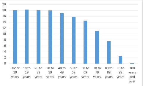
To graph: The histogram for the percentage of the population of the year 2050.

Explanation of Solution

Graph: To obtain the histogram for the obtained result in previous part, Excel is used. The below steps are followed to obtain the required histogram.

Step 1: The data is entered in the Excel worksheet. The snapshot of the obtained table is shown below:

Step 2: Select the data set and go to insert and select the option of cluster column under the Recommended Charts. The screenshot is shown below:

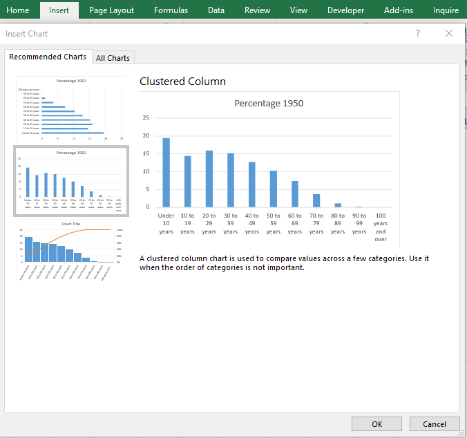
Step 3: Click on OK. The diagram is obtained as follows:

Step 4: Click on the chart area and select the option of “Primary Horizontal” and “Primary Vertical” axis under the “Add Chart Element” to add the axis title. The screenshot is shown below:

Step 5: Click on the bars of the diagrams and reduce the gap width to zero under the “Format Data Series” tab. The screenshot is shown below:

The obtained histogram is as follows:

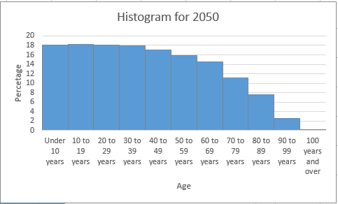
Interpretation: The histogram for the age distribution of the year 2050 shows that percentage of the age groups from under 10 years to 30–39 years are almost equal.

To determine

The change between the age distribution of the year 1950 and 2050.

Answer to Problem 20E

Solution: The main change between the age distribution of the year 1950 and the year 2050 is the amount of the skewness.

Explanation of Solution

The age distribution of the year 1950 is right-skewed. But the histogram for the age distribution of the year 2050 shows that percentage of the age groups from under 10 years to 30–39 years are almost equal. After the age 40, the percentages start to decline. The lowest percentage is in the age group 100 years and more.