
Concept Introduction:
The formula to calculate change in GDP is,
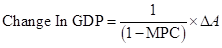
Here,
 is autonomous spending.
 - MPC is marginal propensity to consume.
Marginal Propensity to Consume ( MPC ): It is defined as the change which occurs in total consumption level due to change in disposable income.
The formula to calculate MPC is,

Here,
 is change in disposable income.
  is change in consumption level.
 - MPC is marginal propensity to consume.
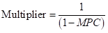
Multiplier: It is defined as the ratio of total change in gross domestic product due to change in the autonomous spending.
The formula to calculate multiplier is,
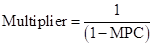
Here,
- MPC is marginal propensity to consume.
Consumption Level ( C ): It is one of the largest components of GDP .The individual consumption Depends on the disposable income.
Consumption Function: It shows how the change in disposable income of an individual changes the consumption level.
The formula to calculate consumption function is,
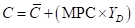
Here,
- C is consumption level.
 is autonomous consumption.
 is disposable income
- MPC is marginal propensity to consume.
Autonomous Consumption: This is defined as the consumption level when the income of an individual is zero.
Planned Aggregate Spending: It is the summation of consumption level in an economy and the planned investment.
The formula to calculate planned aggregate spending is,
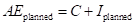
Here,
- C is consumption level.
 is the planned investment spending.
  is the planned aggregate spending.
Unplanned Investment: All those investments that businesses do not intend to take in given time. It is certain due to some external factors like fall in interest rate and increase in future profitability.
The formula to calculate unplanned investment is,
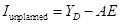
Here,
- YDis disposable income.
 is unplanned investment spending.
 - AE is the planned aggregate spending.
Answer to Problem 13P
a. Planned aggregate expenditure and unplanned investment.
| GDP | YD (A) | C (B) | Iplanned (C ) | AEplanned  | Iunplanned  |
| (billions of dollars) | |||||
| 0 | 0 | 100 | 300 | 400 |  |
| 400 | 400 | 400 | 300 | 700 |  |
| 800 | 800 | 700 | 300 | 1,000 |  |
| 1,200 | 1,200 | 1,000 | 300 | 1,300 |  |
| 1,600 | 1,600 | 1,300 | 300 | 1,600 | 0 |
| 2,000 | 2,000 | 1,600 | 300 | 1,900 | 100 |
| 2,400 | 2,400 | 1,900 | 300 | 2,200 | 200 |
| 2,800 | 2,800 | 2,200 | 300 | 2,500 | 300 |
| 3,200 | 3,200 | 2,500 | 300 | 2,800 | 400 |
b. Aggregate consumption function.
Given,
Autonomous consumption is $100 billion.
Change in disposable income is $400 billion.
Change in aggregate consumer spending is $300 billion.
The formula to calculate MPC is,

Substitute $300 billion for  and $400 billion for
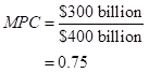
Hence MPC is 0.75.
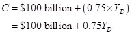
The formula to calculate consumption function is,
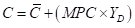
Substitute $100 billion for  and 0.75 for MPC.
c. Income- expenditure equilibrium GDP.
The equilibrium GDP (Y*) is $1,600 billion.
Explanation of Solution
Income expenditure equilibrium GDP is the point where planned aggregate spending is equal to the GDP. The table drawn in part a highlights the condition is satisfied at the level where GDP is equal to $1,600 billion.
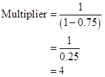
d. Value of the multiplier.
Given,
MPC is 0.75.
The formula to calculate multiplier is,
Substitute 0.75 for MPC.
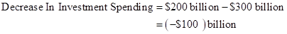
e. The new Y * when planned investment changes.
Given,
New investment is $200 billion.
Initial investment is $300 billion.
The formula to calculate change in planned investment is,

Substitute $200 billion for new investment and $200 billion for initial investment.
Given,
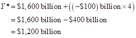
Change in investment is  billion.
Real GDP is $1,600 billion.
Multiplier is 4.
The formula to calculate new Y* is,

Substitute $1,600 billion for real GDP, 4 for multiplier and  billion for change in investment.
f. The new Y * when autonomous consumption changes.
Given,
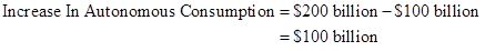
New autonomous consumption is $200 billion.
Initial autonomous consumption is $100 billion.
The formula to calculate change in autonomous consumption is,
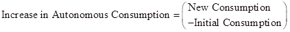
Substitute $200 billion for new consumption and $100 billion for initial consumption.
Given,
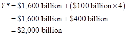
Change in consumption is $100 billion.
Real GDP is $1,600 billion.
Multiplier is 4.
The formula to calculate new Y* is,

Substitute $1,600 billion for real GDP, 4 for multiplier and $100 billion for change in consumption.
Want to see more full solutions like this?
Chapter 11 Solutions
MACROECONOMICS W/ ACHEIVE ACCESS LL

- Use the Feynman technique throughout. Assume that you’re explaining the answer to someone who doesn’t know the topic at all. Write explanation in paragraphs and if you use currency use USD currency: 10. What is the mechanism or process that allows the expenditure multiplier to “work” in theKeynesian Cross Model? Explain and show both mathematically and graphically. What isthe underpinning assumption for the process to transpire?arrow_forwardUse the Feynman technique throughout. Assume that you’reexplaining the answer to someone who doesn’t know the topic at all. Write it all in paragraphs: 2. Give an overview of the equation of exchange (EoE) as used by Classical Theory. Now,carefully explain each variable in the EoE. What is meant by the “quantity theory of money”and how is it different from or the same as the equation of exchange?arrow_forwardZbsbwhjw8272:shbwhahwh Zbsbwhjw8272:shbwhahwh Zbsbwhjw8272:shbwhahwhZbsbwhjw8272:shbwhahwhZbsbwhjw8272:shbwhahwharrow_forward
- Use the Feynman technique throughout. Assume that you’re explaining the answer to someone who doesn’t know the topic at all:arrow_forwardUse the Feynman technique throughout. Assume that you’reexplaining the answer to someone who doesn’t know the topic at all: 4. Draw a Keynesian AD curve in P – Y space and list the shift factors that will shift theKeynesian AD curve upward and to the right. Draw a separate Classical AD curve in P – Yspace and list the shift factors that will shift the Classical AD curve upward and to the right.arrow_forwardUse the Feynman technique throughout. Assume that you’re explaining the answer to someone who doesn’t know the topic at all: 10. What is the mechanism or process that allows the expenditure multiplier to “work” in theKeynesian Cross Model? Explain and show both mathematically and graphically. What isthe underpinning assumption for the process to transpire?arrow_forward
- Use the Feynman technique throughout. Assume that you’re explaining the answer to someone who doesn’t know the topic at all: 15. How is the Keynesian expenditure multiplier implicit in the Keynesian version of the AD/ASmodel? Explain and show mathematically. (note: this is a tough one)arrow_forwardUse the Feynman technique throughout. Assume that you’re explaining the answer to someone who doesn’t know the topic at all: 13. What would happen to the net exports function in Europe and the US respectively if thedemand for dollars rises worldwide? Explain why.arrow_forward20. Given the mathematical model below, solve for the expenditure multiplier for a) government spending, G; and b) for consumer taxes, T. (medium difficulty) Y=C+I+G C=Co+b(Y-T) 1 = 10 T=To+tY G = Go+gYarrow_forward
- Use the Feynman technique throughout. Assume that you’re explaining the answer to someone who doesn’t know the topic at all: 11. What exactly is a rectangular hyperbola and what relevance is it to classical economics?arrow_forwardUse the Feynman technique throughout. Assume that you’re explaining the answer to someone who doesn’t know the topic at all: 9. Explain the difference between absolute and comparative advantage in a family setting, i.e.using parents and children. What can we glean from knowing about comparative andabsolute advantages?arrow_forwardUse the Feynman technique throughout. Assume that you’re explaining the answer to someone who doesn’t know the topic at all: 18. Explain why most economists believe it is absolutely necessary to allow free trade in aneconomy. Why is it harmful (under most circumstances) to have tariffs and trade barriers?arrow_forward

 Principles of Economics (12th Edition)EconomicsISBN:9780134078779Author:Karl E. Case, Ray C. Fair, Sharon E. OsterPublisher:PEARSON
 Engineering Economy (17th Edition)EconomicsISBN:9780134870069Author:William G. Sullivan, Elin M. Wicks, C. Patrick KoellingPublisher:PEARSON
 Principles of Economics (MindTap Course List)EconomicsISBN:9781305585126Author:N. Gregory MankiwPublisher:Cengage Learning
 Managerial Economics: A Problem Solving ApproachEconomicsISBN:9781337106665Author:Luke M. Froeb, Brian T. McCann, Michael R. Ward, Mike ShorPublisher:Cengage Learning
 Managerial Economics & Business Strategy (Mcgraw-...EconomicsISBN:9781259290619Author:Michael Baye, Jeff PrincePublisher:McGraw-Hill Education