
Concept Introduction:
The formula to calculate change in GDP is,
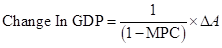
Here,
 is autonomous spending.
 - MPC is marginal propensity to consume.
Marginal Propensity to Consume ( MPC ): It is defined as the change which occurs in total consumption level due to change in disposable income.
The formula to calculate MPC is,

Here,
 is change in disposable income.
  is change in consumption level.
 - MPC is marginal propensity to consume.
Multiplier: It is defined as the ratio of total change in gross domestic product due to change in the autonomous spending.
The formula to calculate multiplier is,
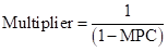
Here,
- MPC is marginal propensity to consume.
Consumption Level ( C ): It is one of the largest components of GDP .The individual consumption Depends on the disposable income.
Consumption Function: It shows how the change in disposable income of an individual changes the consumption level.
The formula to calculate consumption function is,
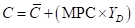
Here,
- C is consumption level.
 is autonomous consumption.
 is disposable income
- MPC is marginal propensity to consume.
Autonomous Consumption: This is defined as the consumption level when the income of an individual is zero.
Planned Aggregate Spending: It is the summation of consumption level in an economy and the planned investment.
The formula to calculate planned aggregate spending is,
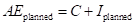
Here,
- C is consumption level.
 is the planned investment spending.
  is the planned aggregate spending.
Unplanned Investment: All those investments that businesses do not intend to take in given time. It is certain due to some external factors like fall in interest rate and increase in future profitability.
The formula to calculate unplanned investment is,
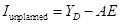
Here,
- YDis disposable income.
 is unplanned investment spending.
 - AE is the planned aggregate spending.
Answer to Problem 13P
a. Planned aggregate expenditure and unplanned investment.
| GDP | YD (A) | C (B) | Iplanned (C ) | AEplanned  | Iunplanned  |
| (billions of dollars) | |||||
| 0 | 0 | 100 | 300 | 400 |  |
| 400 | 400 | 400 | 300 | 700 |  |
| 800 | 800 | 700 | 300 | 1,000 |  |
| 1,200 | 1,200 | 1,000 | 300 | 1,300 |  |
| 1,600 | 1,600 | 1,300 | 300 | 1,600 | 0 |
| 2,000 | 2,000 | 1,600 | 300 | 1,900 | 100 |
| 2,400 | 2,400 | 1,900 | 300 | 2,200 | 200 |
| 2,800 | 2,800 | 2,200 | 300 | 2,500 | 300 |
| 3,200 | 3,200 | 2,500 | 300 | 2,800 | 400 |
b. Aggregate consumption function.
Given,
Autonomous consumption is $100 billion.
Change in disposable income is $400 billion.
Change in aggregate consumer spending is $300 billion.
The formula to calculate MPC is,

Substitute $300 billion for  and $400 billion for
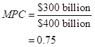
Hence MPC is 0.75.
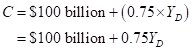
The formula to calculate consumption function is,
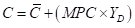
Substitute $100 billion for  and 0.75 for MPC.
c. Income- expenditure equilibrium GDP.
The equilibrium GDP (Y*) is $1,600 billion.
Explanation of Solution
Income expenditure equilibrium GDP is the point where planned aggregate spending is equal to the GDP. The table drawn in part a highlights the condition is satisfied at the level where GDP is equal to $1,600 billion.
d. Value of the multiplier.
Given,
MPC is 0.75.
The formula to calculate multiplier is,
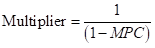
Substitute 0.75 for MPC.
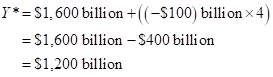
e. The new Y * when planned investment changes.
Given,
New investment is $200 billion.
Initial investment is $300 billion.
The formula to calculate change in planned investment is,

Substitute $200 billion for new investment and $200 billion for initial investment.
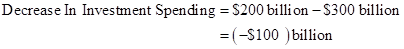
Given,
Change in investment is  billion.
Real GDP is $1,600 billion.
Multiplier is 4.
The formula to calculate new Y* is,

Substitute $1,600 billion for real GDP, 4 for multiplier and  billion for change in investment.
f. The new Y * when autonomous consumption changes.
Given,
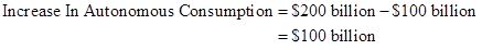
New autonomous consumption is $200 billion.
Initial autonomous consumption is $100 billion.
The formula to calculate change in autonomous consumption is,
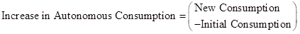
Substitute $200 billion for new consumption and $100 billion for initial consumption.
Given,
Change in consumption is $100 billion.
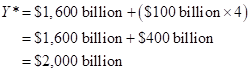
Real GDP is $1,600 billion.
Multiplier is 4.
The formula to calculate new Y* is,

Substitute $1,600 billion for real GDP, 4 for multiplier and $100 billion for change in consumption.
Want to see more full solutions like this?

- I need help in seeing how these are the answers. If you could please write down your steps so I can see how it's done please.arrow_forwardSuppose that a random sample of 216 twenty-year-old men is selected from a population and that their heights and weights are recorded. A regression of weight on height yields Weight = (-107.3628) + 4.2552 x Height, R2 = 0.875, SER = 11.0160 (2.3220) (0.3348) where Weight is measured in pounds and Height is measured in inches. A man has a late growth spurt and grows 1.6200 inches over the course of a year. Construct a confidence interval of 90% for the person's weight gain. The 90% confidence interval for the person's weight gain is ( ☐ ☐) (in pounds). (Round your responses to two decimal places.)arrow_forwardSuppose that (Y, X) satisfy the assumptions specified here. A random sample of n = 498 is drawn and yields Ŷ= 6.47 + 5.66X, R2 = 0.83, SER = 5.3 (3.7) (3.4) Where the numbers in parentheses are the standard errors of the estimated coefficients B₁ = 6.47 and B₁ = 5.66 respectively. Suppose you wanted to test that B₁ is zero at the 5% level. That is, Ho: B₁ = 0 vs. H₁: B₁ #0 Report the t-statistic and p-value for this test. Definition The t-statistic is (Round your response to two decimal places) ☑ The Least Squares Assumptions Y=Bo+B₁X+u, i = 1,..., n, where 1. The error term u; has conditional mean zero given X;: E (u;|X;) = 0; 2. (Y;, X¡), i = 1,..., n, are independent and identically distributed (i.i.d.) draws from i their joint distribution; and 3. Large outliers are unlikely: X; and Y, have nonzero finite fourth moments.arrow_forward
- Asap pleasearrow_forwardTasks Exercise 1 Assess the following functions: 1. f(x)= x2+6x+2 2.f '(x)=10x-2x2+5 a. Find the stationary points. (5 marks) b. Determine whether the stationary point is a maximum or minimum. (5 marks) c. Draw the corresponding curves (5 marks)arrow_forwardProblem 2: The sales data over the last 10 years for the Acme Hardware Store are as follows: 2003 $230,000 2008 $526,000 2004 276,000 2009 605,000 2005 328,000 2010 690,000 2006 388,000 2011 779,000 2007 453,000 2012 873,000 1. Calculate the compound growth rate for the period of 2003 to 2012. 2. Based on your answer to part a, forecast sales for both 2013 and 2014. 3. Now calculate the compound growth rate for the period of 2007 to 2012. 1. Based on your answer to part e, forecast sales for both 2013 and 2014. 5. What is the major reason for the differences in your answers to parts b and d? If you were to make your own projections, what would you forecast? (Drawing a graph is very helpful.)arrow_forward
- Exercise 4A firm has the following average cost: AC = 200 + 2Q – 36 Q Find the stationary point and determine if it is a maximum or a minimum.b. Find the marginal cost function.arrow_forwardExercise 4A firm has the following average cost: AC = 200 + 2Q – 36 Q Find the stationary point and determine if it is a maximum or a minimum.b. Find the marginal cost function.arrow_forwardExercise 2A firm has the following short-run production function: Q = 30L2 -0.5L3a. Make a table with two columns: Production and Labour b. Add a third column to the table with the marginal product of labour c. Graph the values that you estimated for the production function and the marginal product oflabour Exercise 3A Firm has the following production function: Q= 20L-0.4L2a. Using differential calculus find the unit of labour that maximizes the production. b. Estimate function of Marginal product of labor c. Obtain the Average product of labor. d. Find the point at which the Marginal Product of Labour is equal to the Average Product of Labour.arrow_forward
- Problem 3 You have the following data for the last 12 months' sales for the PRQ Corporation (in thousands of dollars): January 500 July 610 February 520 August 620 March 520 September 580 April 510 October 550 May 530 November 510 June 580 December 480 1. Calculate a 3-month centered moving average. 2. Use this moving average to forecast sales for January of next year. 3. If you were asked to forecast January and February sales for next year, would you be confident of your forecast using the preceding moving averages? Why or why not? expect? Explain.arrow_forwardProblem 5 The MNO Corporation is preparing for its stockholder meeting on May 15, 2013. It sent out proxies to its stockholders on March 15 and asked stockholders who plan to attend the meeting to respond. To plan for a sufficient number of information packages to be distributed at the meeting, as well as for refreshments to be served, the company has asked you to forecast the number of attending stockholders. By April 15, 378 stockholders have expressed their intention to attend. You have available the following data for the last 6 years for total attendance at the stockholder meeting and the number of positive responses as of April 15: Year Positive Responses Attendance 2007 322 520 2008 301 550 2009 398 570 2010 421 600 2011 357 570 2012 452 650 1. What is your attendance forecast for the 2013 stockholder meeting? 2. Are there any other factors that could affect attendance, and thus make your forecast inac- curate?arrow_forwardProblem 4 Office Enterprises (OE) produces a line of metal office file cabinets. The company's economist, having investigated a large number of past data, has established the following equation of demand for these cabinets: Q=10,000+6013-100P+50C Q=Annual number of cabinets sold B = Index of nonresidential construction P = Average price per cabinet charged by OE C=Average price per cabinet charged by OE's closest competitor It is expected that next year's nonresidential construction index will stand at 160, OE's average price will be $40, and the competitor's average price will be $35. 1. Forecast next year's sales. 2. What will be the effect if the competitor lowers its price to 832? If it raises its price to $36? 3. What will happen if OE reacts to the decrease mentioned in part b by lowering its price to $37? 4. If the index forecast was wrong, and it turns out to be only 140 next year, what will be the effect on OE's sales? If not, what does it measure?arrow_forward

 Principles of Economics (12th Edition)EconomicsISBN:9780134078779Author:Karl E. Case, Ray C. Fair, Sharon E. OsterPublisher:PEARSON
 Engineering Economy (17th Edition)EconomicsISBN:9780134870069Author:William G. Sullivan, Elin M. Wicks, C. Patrick KoellingPublisher:PEARSON
 Principles of Economics (MindTap Course List)EconomicsISBN:9781305585126Author:N. Gregory MankiwPublisher:Cengage Learning
 Managerial Economics: A Problem Solving ApproachEconomicsISBN:9781337106665Author:Luke M. Froeb, Brian T. McCann, Michael R. Ward, Mike ShorPublisher:Cengage Learning
 Managerial Economics & Business Strategy (Mcgraw-...EconomicsISBN:9781259290619Author:Michael Baye, Jeff PrincePublisher:McGraw-Hill Education