
Concept explainers
Videos
For Exercises 1 through 10, follow these steps.
a. State the hypotheses and identify the claim.
b. Find the critical value(s).
c. Compute the test value.
d. Make the decision.
e. Summarize the results.
Use the traditional method of hypothesis testing unless otherwise specified. Assume all assumptions have been met.
1. Traffic Accident Fatalities A traffic safety report indicated that for the 21–24 year age group, 31.58% of traffic fatalities were victims who had used a seat belt. Victims who were not wearing a seat belt accounted for 59.83% of the deaths, and the status of the rest was unknown. A study of 120 randomly selected traffic fatalities in a particular region showed that for this age group, 35 of the victims had used a seat belt, 78 had not, and the status of the rest was unknown. At α = 0.05, is there sufficient evidence that the proportions differ from those in the report?
Source: New York Times Almanac.
(a)
To state: The hypothesis and the claim.
Answer to Problem 11.1.1RE
The null and alternative hypotheses are:
And the claim of the test is the observed proportion is different from the reported proportion.
Explanation of Solution
Given info:
The percentage of death and the observed count corresponding to each reason are provided in the question. The level of significance is
Justification:
The researcher wants to know that whether the proportion of the traffic fatalities corresponding to each reason is different from the reported proportion or not. The null and alternative hypothesis can be defined as:
Null hypothesis:
Alternative hypothesis:
In the provided situation, the claim of the study will be the observed proportion corresponding to each reason is different from the reported proportion.
(b)
The critical value.
Answer to Problem 11.1.1RE
The required critical value is 5.991.
Explanation of Solution
The required critical value is obtained from the provided chi-square table in the textbook. The number of categories is 3.
The degrees of freedom is calculated as:
Therefore, the critical value at
(c)
The value of the test statistic.
Answer to Problem 11.1.1RE
The test statistic value is 1.819.
Explanation of Solution
Calculation:
Software procedure:
Step-by-step procedure to obtain the test statistic using the MINITAB software:
- Enter the data in the Minitab worksheet.
- Go to Stat> Tables> Chi-Square Goodness-of-Fit Test (one variable).
- Specify the “Observed count”, choose the option “Proportions specified by historic count”, and specify the column where the percentage is written.
- Click on OK.
Output using the MINITAB software is given below:
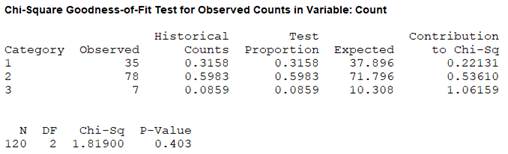
Therefore, the obtained value of the test statistic is 1.819.
(d)
To make: The decision.
Answer to Problem 11.1.1RE
The null hypothesis will not be rejected.
Explanation of Solution
The obtained value of the test statistic is 1.819 and the critical value is 5.991. As the obtained value of the chi-square statistic is less than the critical value, it can be said that there is not enough evidence to reject the null hypothesis at
(e)
To summarize: The results.
Answer to Problem 11.1.1RE
According to the obtained result, the claim of the study is not true.
Explanation of Solution
The null hypothesis is not rejected. On the basis of the obtained result, it can be concluded that the result of the proportion of the traffic fatalities is not different from the reported proportion at
Want to see more full solutions like this?
Chapter 11 Solutions
Elementary Statistics: A Step By Step Approach


- A special interest group reports a tiny margin of error (plus or minus 0.04 percent) for its online survey based on 50,000 responses. Is the margin of error legitimate? (Assume that the group’s math is correct.)arrow_forwardSuppose that 73 percent of a sample of 1,000 U.S. college students drive a used car as opposed to a new car or no car at all. Find an 80 percent confidence interval for the percentage of all U.S. college students who drive a used car.What sample size would cut this margin of error in half?arrow_forwardYou want to compare the average number of tines on the antlers of male deer in two nearby metro parks. A sample of 30 deer from the first park shows an average of 5 tines with a population standard deviation of 3. A sample of 35 deer from the second park shows an average of 6 tines with a population standard deviation of 3.2. Find a 95 percent confidence interval for the difference in average number of tines for all male deer in the two metro parks (second park minus first park).Do the parks’ deer populations differ in average size of deer antlers?arrow_forward
- Suppose that you want to increase the confidence level of a particular confidence interval from 80 percent to 95 percent without changing the width of the confidence interval. Can you do it?arrow_forwardA random sample of 1,117 U.S. college students finds that 729 go home at least once each term. Find a 98 percent confidence interval for the proportion of all U.S. college students who go home at least once each term.arrow_forwardSuppose that you make two confidence intervals with the same data set — one with a 95 percent confidence level and the other with a 99.7 percent confidence level. Which interval is wider?Is a wide confidence interval a good thing?arrow_forward
- Is it true that a 95 percent confidence interval means you’re 95 percent confident that the sample statistic is in the interval?arrow_forwardTines can range from 2 to upwards of 50 or more on a male deer. You want to estimate the average number of tines on the antlers of male deer in a nearby metro park. A sample of 30 deer has an average of 5 tines, with a population standard deviation of 3. Find a 95 percent confidence interval for the average number of tines for all male deer in this metro park.Find a 98 percent confidence interval for the average number of tines for all male deer in this metro park.arrow_forwardBased on a sample of 100 participants, the average weight loss the first month under a new (competing) weight-loss plan is 11.4 pounds with a population standard deviation of 5.1 pounds. The average weight loss for the first month for 100 people on the old (standard) weight-loss plan is 12.8 pounds, with population standard deviation of 4.8 pounds. Find a 90 percent confidence interval for the difference in weight loss for the two plans( old minus new) Whats the margin of error for your calculated confidence interval?arrow_forward
- A 95 percent confidence interval for the average miles per gallon for all cars of a certain type is 32.1, plus or minus 1.8. The interval is based on a sample of 40 randomly selected cars. What units represent the margin of error?Suppose that you want to decrease the margin of error, but you want to keep 95 percent confidence. What should you do?arrow_forward3. (i) Below is the R code for performing a X2 test on a 2×3 matrix of categorical variables called TestMatrix: chisq.test(Test Matrix) (a) Assuming we have a significant result for this procedure, provide the R code (including any required packages) for an appropriate post hoc test. (b) If we were to apply this technique to a 2 × 2 case, how would we adapt the code in order to perform the correct test? (ii) What procedure can we use if we want to test for association when we have ordinal variables? What code do we use in R to do this? What package does this command belong to? (iii) The following code contains the initial steps for a scenario where we are looking to investigate the relationship between age and whether someone owns a car by using frequencies. There are two issues with the code - please state these. Row3<-c(75,15) Row4<-c(50,-10) MortgageMatrix<-matrix(c(Row1, Row4), byrow=T, nrow=2, MortgageMatrix dimnames=list(c("Yes", "No"), c("40 or older","<40")))…arrow_forwardDescribe the situation in which Fisher’s exact test would be used?(ii) When do we use Yates’ continuity correction (with respect to contingencytables)?[2 Marks] 2. Investigate, checking the relevant assumptions, whether there is an associationbetween age group and home ownership based on the sample dataset for atown below:Home Owner: Yes NoUnder 40 39 12140 and over 181 59Calculate and evaluate the effect size.arrow_forward
 Glencoe Algebra 1, Student Edition, 9780079039897...AlgebraISBN:9780079039897Author:CarterPublisher:McGraw Hill
 College Algebra (MindTap Course List)AlgebraISBN:9781305652231Author:R. David Gustafson, Jeff HughesPublisher:Cengage Learning
 Holt Mcdougal Larson Pre-algebra: Student Edition...AlgebraISBN:9780547587776Author:HOLT MCDOUGALPublisher:HOLT MCDOUGAL