Chapter 10.5, Problem 15E

To determine

To perform:

A hypothesis test.

Answer to Problem 15E

Solution:

a. $H_0:{\sigma }^2=2.25$; $H_a:{\sigma }^2\ne 2.25$

b. Chi- square distribution; $\alpha =0.10$

c. ${\chi }^2=23.7067$

d. ${\chi }_{0.95}^2=\begin{array}{l}6.5706\hfill \end{array}$, ${\chi }_{0.05}^2=\begin{array}{l}\begin{array}{l}\begin{array}{l}23.6850\hfill \end{array}\hfill \end{array}\hfill \end{array}$. Therefore, the decision rule is to reject the null hypothesis $H_0$ if ${\chi }^2\le 6.5106or{\chi }^2\ge 23.6850$. There is sufficient evidence to support the manager’s claim that the variance in the water temperature is no longer 2.25.

Explanation of Solution

Consider the following scenario,

“A health club needs to ensure that the temperature in its heated pool stays constant throughout the winter months. Otherwise it needs to invest in a new heater for the pool. It is assumed that the daily water temperatures, measured in degrees Fahrenheit $\left({}^{\circ }F\right)$, have a varience of 2.25, which is considered to be within normal limits for a properly operating heater. The pool manager needs to determine if the variance is still 2.25, so she perform a hypothesis test to test the claim that the variance in the temperature is not 2.25. after testing the pool water for a random sample of 15 winter days, the pool manager finds a mean daily temperature of ${78.60}^{\circ }F$ with a variance of 3.81.”.

a: State the null and alternative hypothesis.

Suppose pool manager claims that variance in the temperature is not 2.25. That is the research hypothesis $H_a$ is that the variance is not 2.25 which is wrriten mathematically as ${\sigma }^2\ne 2.25$. The logical opposite is ${\sigma }^2=2.25$. Thus the hypotheses are tested as follows,

The Null hypothesis:$H_0:{\sigma }^2=2.25$

The altenative hypotheis: $H_a:{\sigma }^2\ne 2.25$

b: Determine which distribution to use for the test statistic, and state the level of significance.

Since we are testing a population variance and we are told we can safely assume that all necessary conditions are met, we can use the chi- square distribution and thus the ${\chi }^2$-test statistic with the given level of significance of $\alpha =0.10$.

c: Gather data and calculate the necessary sample statistics.

The test statistic formula:

Test statistic for a hypothesis test for a population variance or population stadard deviation

When the sample taken is a simple random sample and the population distribution is approximately normal, the test statistic for a hypothesis test for a population variance or population standard deviation is given by,

${\chi }^2=\frac{\left(n-1\right)s^2}{{\sigma }^2}$

Where n is the sample size,

$s^2$ is the sample variance, and

${\sigma }^2$ is the presumed value of the population variance (or square of the prsumed value of the population standard deviation) from the null hypothesis

The given information is,

$n=15,s^2=3.81and{\sigma }^2=2.25$.

Substitute these values in the test statistic formula to get the following,

$\begin{array}{rll}{\chi }^2& =& \frac{\left(n-1\right)s^2}{{\sigma }^2}\\ & =& \frac{\left(15-1\right)\times 3.81}{2.25}\\ & =& \frac{14\times 3.81}{2.25}\\ & =& \frac{53.34}{2.25}\\ & =& 23.7067\end{array}$

d: Draw a conclusion and interpret the decision.

Rejection Region for Hypothesis Tests for Population Variances and Standard Deviations:

Reject the null hypothesis, $H_0$, if

${\chi }^2\le {\chi }_{\left(1-\alpha \right)}^2$ for a left-tailed test

${\chi }^2\ge {\chi }_{\alpha }^2$ for a right-tailed test

${\chi }^2\le {\chi }_{\left(1-\alpha /2\right)}^{2}or{\chi }^2\ge {\chi }_{\alpha /2}^2$ for a two-tailed test.

Degrees of Freedom for a Hypothesis Test for a Population Variance or Population Standard Deviation

In a hypothesis test for a population variance or population standard deviation the number of degrees of freedom for the chi- square distribution of the test statistic is given by

$df=n-1$

Where n is the sample size.

Form the given information this is the two-tailed test since $H_a:{\sigma }^2\ne 2.25$ so the rejection region is ${\chi }^2\le {\chi }_{\left(1-\alpha /2\right)}^{2}or{\chi }^2\ge {\chi }_{\alpha /2}^2$.

From the given information n = 15.

The degrees of freedom is given below,

$\begin{array}{rll}df& =& n-1\\ & =& 15-1\\ & =& 14\end{array}$

Conclusion:

Use the level of significance of $\alpha =0.10$ to find the critical value ${\chi }_{\left(1-\alpha /2\right)}^2={\chi }_{\left(1-0.10/2\right)}^2={\chi }_{\left(1-0.05\right)}^2={\chi }_{0.95}^2$ of the chi-square distribution with df = 14 in order to make a decision about the null hypothesis.

Use the “Area to the right of the critical value ${\chi }^2$” table to get the following,

${\chi }_{0.95}^2=\begin{array}{l}6.5706\hfill \end{array}$

Use the level of significance of $\alpha =0.05$ to find the critical value ${\chi }_{\alpha /2}^2={\chi }_{0.1/2}^2={\chi }_{0.05}^2$ of the chi-square distribution with df = 14 in order to make a decision about the null hypothesis.

Use the “Area to the right of the critical value ${\chi }^2$” table to get the following,

${\chi }_{0.05}^2=\begin{array}{l}\begin{array}{l}\begin{array}{l}23.6850\hfill \end{array}\hfill \end{array}\hfill \end{array}$

Therefore, the decision rule is to reject the null hypothesis $H_0$ if ${\chi }^2\le 6.5106or{\chi }^2\ge 23.6850$.

So, the left-hand critical value of the test statistic is ${\chi }_{0.95}^2\le 6.5706$ and right-hand critical value is ${\chi }_{0.05}^2\ge 23.6850$.

The calculated test statistic is ${\chi }^2=23.7067$.

The diagrammatic representation is given below,

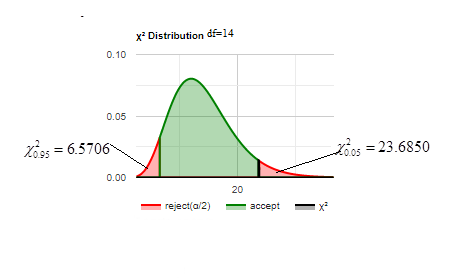
By using the above condition we reject the null hypothesis.

Since $23.7067>6.5106or23.7067>23.6850$.

So, there is sufficient evidence to support the manager’s claim that the variance in the water temperature is no longer 2.25.

Final statement:

There is sufficient evidence to support the manager’s claim that the variance in the water temperature is no longer 2.25.