6th Edition

ISBN: 9781323845820

Author: Triola

Publisher: PEARSON

Concept explainers

Correlation defines a relationship between two independent variables. It tells the degree to which variables move in relation to each other. When two sets of data are related to each other, there is a correlation between them.

Linear Correlation

A correlation is used to determine the relationships between numerical and categorical variables. In other words, it is an indicator of how things are connected to one another. The correlation analysis is the study of how variables are related.

Regression Analysis

Regression analysis is a statistical method in which it estimates the relationship between a dependent variable and one or more independent variable. In simple terms dependent variable is called as outcome variable and independent variable is called as p…

Videos

Textbook Question

Chapter 10.2, Problem 19BSC

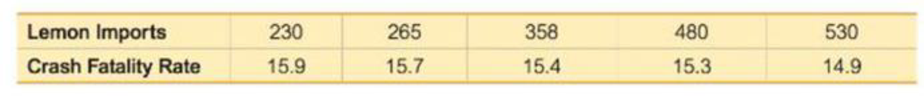
Regression and Predictions. Exercises 13–28 use the same data sets as Exercises 13–28 in Section 10-1. In each case, find the regression equation, letting the first variable be the predictor (x) variable, Find the indicated predicted value by following the prediction procedure summarized in Figure 10-5 on page 493.

19. Lemons and Car Crashes Using the listed lemon/crash data, find the best predicted crash fatality rate for a year in which there are 500 metric tons of lemon imports. Is the prediction worthwhile?

Chapter 10.2, Problem 19BSC, Regression and Predictions. Exercises 1328 use the same data sets as Exercises 1328 in Section 10-1.

Expert Solution & Answer

Want to see the full answer?

Check out a sample textbook solution

See solution

Chapter 10.2, Problem 18BSC

Chapter 10.2, Problem 20BSC

Students have asked these similar questions

2 (VaR and ES) Suppose X1 are independent. Prove that ~ Unif[-0.5, 0.5] and X2 VaRa (X1X2) < VaRa(X1) + VaRa (X2). ~ Unif[-0.5, 0.5]

8 (Correlation and Diversification) Assume we have two stocks, A and B, show that a particular combination of the two stocks produce a risk-free portfolio when the correlation between the return of A and B is -1.

9 (Portfolio allocation) Suppose R₁ and R2 are returns of 2 assets and with expected return and variance respectively r₁ and 72 and variance-covariance σ2, 0%½ and σ12. Find −∞ ≤ w ≤ ∞ such that the portfolio wR₁ + (1 - w) R₂ has the smallest risk.

Chapter 10 Solutions

ESSENTIALS OF STATISTICS 6TH ED W/MYSTA

Ch. 10.1 - Notation Twenty different statistics students are...Ch. 10.1 - Interpreting r For the some two variables...Ch. 10.1 - Global Warming If we find that there is a linear...Ch. 10.1 - Scatterplots Match these values of r with the five...Ch. 10.1 - Bear Weight and Chest Size Fifty-four wild bears...Ch. 10.1 - Casino Size and Revenue The New York Times...Ch. 10.1 - Garbage Data Set 31 Garbage Weight in Appendix B...Ch. 10.1 - Cereal Killers The amounts of sugar (grams of...Ch. 10.1 - Explore! Exercises 9 and 10 provide two data sets...Ch. 10.1 - Explore! Exercises 9 and 10 provide two data sets...

Knowledge Booster

$Statistics$

Learn more about

Need a deep-dive on the concept behind this application? Look no further. Learn more about this topic, statistics and related others by exploring similar questions and additional content below.