
Concept explainers
Videos
Stopping Distances
In a study on speed control, it was found that the main reasons for regulations were to make traffic flow more efficient and to minimize the risk of danger. An area that was focused on in the study was the distance required to completely stop a vehicle at various speeds. Use the following table to answer the questions.
| MPH | Braking distance (feet) |
| 20 30 40 50 60 80 |
20 45 81 133 205 411 |
Assume MPH is going to be used to predict stopping distance.
1. Which of the two variables is the independent variable?
2. Which is the dependent variable?
3. What type of variable is the independent variable?
4. What type of variable is the dependent variable?
5. Construct a
6. Is there a linear relationship between the two variables?
7. Redraw the scatter plot, and change the distances between the independent-variable numbers. Does the relationship look different?
8. Is the relationship positive or negative?
9. Can braking distance be accurately predicted from MPH?
10.List some other variables that affect braking distance.
11. Compute the value of r.
12. Is r significant at α = 0.05?
1.
To identify: The independent variable.
Answer to Problem 1AC
The independent variable is MPH (miles per hour).
Explanation of Solution
Given info:
The table shows the MPH (miles per hour) and Braking distance in feet.
Calculation:
Independent variable:
If the variable does not dependent on the other variables then the variables are said to be independent variable.
Here, the variable “Miles per hour” does not depend on the other variables. Thus, the independent variable is MPH (miles per hour).
2.
To identify: The dependent variable.
Answer to Problem 1AC
The dependent variable is Braking distance (feet).
Explanation of Solution
Calculation:
Dependent variable:
If the variable depends on the other variables then the variable is said to be dependent variable.
Here, the variable “Braking distance” depends on the other variables. That is the variable braking distance depends on the MPH (miles per hour). Thus, the dependent variable is Braking distance (feet).
3.
The type of variable is the independent variable.
Answer to Problem 1AC
The type of independent variable is the continuous quantitative variable.
Explanation of Solution
Justification:
Continuous quantitative variable:
If the variable takes values on interval scale then the variable is said to be continuous quantitative variable. In the continuous variable, the infinitely many number of values can be considered.
Here, the independent variable miles per hour (MPH) can take any value from a wide range of values. Thus, the independent variable miles per hour (MPH) is continuous quantitative variable.
4.
The type of variable is the dependent variable.
Answer to Problem 1AC
The type of dependent variable is the continuous quantitative variable.
Explanation of Solution
Justification:
Here, the dependent variable braking distance (feet) can take any value from a wide range of values. Thus, the independent variable braking distance (feet) is continuous quantitative variable.
5.
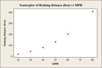
To construct: The scatterplot for the data.
Answer to Problem 1AC
The scatterplot for the data given data using Minitab software is:
Explanation of Solution
Calculation:
The data shows the MPH (miles per hour) and Braking distance (feet) for vehicles.
Step by step procedure to obtain scatterplot using the MINITAB software:
- Choose Graph > Scatterplot.
- Choose Simple and then click OK.
- Under Y variables, enter a column of Braking distance (feet).
- Under X variables, enter a column of MPH.
- Click OK.
6.
To check: Whether there is a linear relationship between the two variables.
Answer to Problem 1AC
Yes, there is a linear relationship between the two variables.
Explanation of Solution
Justification:
The horizontal axis represents miles per hour (MPH) and vertical axis represents braking distance (feet).
From the plot, it is observed that there is a linear relationship between the variables miles per hour (MPH) and braking distance (feet) because the data points show a distinct pattern.
7.
To construct: The scatterplot for the changed data.
To check: Whether the relationship looks different or not.
Answer to Problem 1AC
The scatterplot for the changed data by using Minitab software is:
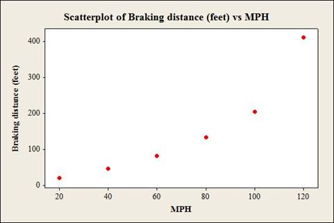
The increments will change the appearance of the relationship if changing the distance between the independent-variable (mph).
Explanation of Solution
Calculation:
The data shows the MPH (miles per hour) and Braking distance (feet) for vehicles.
After changing the distance between the independent-variable numbers, the number of the independent-variable is, 20, 40, 60, 80, 100 and 120.
Step by step procedure to obtain scatterplot using the MINITAB software:
- Choose Graph > Scatterplot.
- Choose Simple and then click OK.
- Under Y variables, enter a column of Braking distance (feet).
- Under X variables, enter a column of MPH.
- Click OK.
Justification:
From the graphs it can be observed that, after changing the distance between the independent-variable (mph), the increments will change the appearance of the relationship.
8.
To check: Whether the relationship is positive or negative.
Answer to Problem 1AC
The relationship is positive.
Explanation of Solution
Justification:
The relationship is positive because the values of independent variable increases then the values of corresponding dependent variable are increases.
9.
To check: Whether the braking distance can be accurately predicted from MPH.
Answer to Problem 1AC
Yes, the braking distance can be accurately predicted from MPH.
Explanation of Solution
Justification:
Here, the braking distance can be accurately predicted from MPH because the relationship between two variables MPH and Breaking distance is strong.
10.
To list: The other variables that affect braking distance.
Answer to Problem 1AC
The other variables that affect braking distance are road conditions, driver response time and condition of the brakes.
Explanation of Solution
Justification:
Answer may wary. One of the possible answers is as follows.
The variable affecting the braking distance are road conditions, driver response time and condition of the brakes.
11.
To compute: The value of r.
Answer to Problem 1AC
The value of r is 0.966.
Explanation of Solution
Calculation:
Correlation coefficient r:
Software Procedure:
Step-by-step procedure to obtain the ‘correlation coefficient’ using the MINITAB software:
- Select Stat > Basic Statistics > Correlation.
- In Variables, select MPH and Braking distance (feet) from the box on the left.
- Click OK.
Output using the MINITAB software is given below:
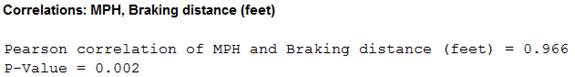
Thus, the Pearson correlation of MPH and Braking distance is 0.966.
12.
To check: Whether or not the r value is significant at 0.05.
Answer to Problem 1AC
Yes, the r value is significant at 0.05.
Explanation of Solution
Calculation:
Here, the r value is significant is checked. So, the claim is that the r value is significant.
The hypotheses are given below:
Null hypothesis:
That is, there is no linear relation between the MPH and Braking distance.
Alternative hypothesis:
That is, there is linear relation between the MPH and Braking distance.
The sample size is 6.
The formula to find the degrees of the freedom is
That is,
From the “TABLE –I: Critical Values for the PPMC”, the critical value for 4 degrees of freedom and
Rejection Rule:
If the absolute value of r is greater than the critical value then reject the null hypothesis.
Conclusion:
From part (11), the Pearson correlation of MPH and Braking distance is 0.966. That is the absolute value of r is 0.966.
Here,
By the rejection rule, reject the null hypothesis.
There is sufficient evidence to support the claim that “there is a linear relation between the MPH and Braking distance”.
Want to see more full solutions like this?
Chapter 10 Solutions
Connect Plus Statistics Hosted by ALEKS Access Card 52 Weeks for Elementary Statistics: A Step-By-St
Additional Math Textbook Solutions
Introductory Statistics
Elementary & Intermediate Algebra
A First Course in Probability (10th Edition)
Calculus: Early Transcendentals (2nd Edition)
Elementary Statistics: Picturing the World (7th Edition)
Basic College Mathematics


- 1 No. 2 3 4 Binomial Prob. X n P Answer 5 6 4 7 8 9 10 12345678 8 3 4 2 2552 10 0.7 0.233 0.3 0.132 7 0.6 0.290 20 0.02 0.053 150 1000 0.15 0.035 8 7 10 0.7 0.383 11 9 3 5 0.3 0.132 12 10 4 7 0.6 0.290 13 Poisson Probability 14 X lambda Answer 18 4 19 20 21 22 23 9 15 16 17 3 1234567829 3 2 0.180 2 1.5 0.251 12 10 0.095 5 3 0.101 7 4 0.060 3 2 0.180 2 1.5 0.251 24 10 12 10 0.095arrow_forwardstep by step on Microssoft on how to put this in excel and the answers please Find binomial probability if: x = 8, n = 10, p = 0.7 x= 3, n=5, p = 0.3 x = 4, n=7, p = 0.6 Quality Control: A factory produces light bulbs with a 2% defect rate. If a random sample of 20 bulbs is tested, what is the probability that exactly 2 bulbs are defective? (hint: p=2% or 0.02; x =2, n=20; use the same logic for the following problems) Marketing Campaign: A marketing company sends out 1,000 promotional emails. The probability of any email being opened is 0.15. What is the probability that exactly 150 emails will be opened? (hint: total emails or n=1000, x =150) Customer Satisfaction: A survey shows that 70% of customers are satisfied with a new product. Out of 10 randomly selected customers, what is the probability that at least 8 are satisfied? (hint: One of the keyword in this question is “at least 8”, it is not “exactly 8”, the correct formula for this should be = 1- (binom.dist(7, 10, 0.7,…arrow_forwardKate, Luke, Mary and Nancy are sharing a cake. The cake had previously been divided into four slices (s1, s2, s3 and s4). What is an example of fair division of the cake S1 S2 S3 S4 Kate $4.00 $6.00 $6.00 $4.00 Luke $5.30 $5.00 $5.25 $5.45 Mary $4.25 $4.50 $3.50 $3.75 Nancy $6.00 $4.00 $4.00 $6.00arrow_forward
- Faye cuts the sandwich in two fair shares to her. What is the first half s1arrow_forwardQuestion 2. An American option on a stock has payoff given by F = f(St) when it is exercised at time t. We know that the function f is convex. A person claims that because of convexity, it is optimal to exercise at expiration T. Do you agree with them?arrow_forwardQuestion 4. We consider a CRR model with So == 5 and up and down factors u = 1.03 and d = 0.96. We consider the interest rate r = 4% (over one period). Is this a suitable CRR model? (Explain your answer.)arrow_forward
- Question 3. We want to price a put option with strike price K and expiration T. Two financial advisors estimate the parameters with two different statistical methods: they obtain the same return rate μ, the same volatility σ, but the first advisor has interest r₁ and the second advisor has interest rate r2 (r1>r2). They both use a CRR model with the same number of periods to price the option. Which advisor will get the larger price? (Explain your answer.)arrow_forwardQuestion 5. We consider a put option with strike price K and expiration T. This option is priced using a 1-period CRR model. We consider r > 0, and σ > 0 very large. What is the approximate price of the option? In other words, what is the limit of the price of the option as σ∞. (Briefly justify your answer.)arrow_forwardQuestion 6. You collect daily data for the stock of a company Z over the past 4 months (i.e. 80 days) and calculate the log-returns (yk)/(-1. You want to build a CRR model for the evolution of the stock. The expected value and standard deviation of the log-returns are y = 0.06 and Sy 0.1. The money market interest rate is r = 0.04. Determine the risk-neutral probability of the model.arrow_forward
- Several markets (Japan, Switzerland) introduced negative interest rates on their money market. In this problem, we will consider an annual interest rate r < 0. We consider a stock modeled by an N-period CRR model where each period is 1 year (At = 1) and the up and down factors are u and d. (a) We consider an American put option with strike price K and expiration T. Prove that if <0, the optimal strategy is to wait until expiration T to exercise.arrow_forwardWe consider an N-period CRR model where each period is 1 year (At = 1), the up factor is u = 0.1, the down factor is d = e−0.3 and r = 0. We remind you that in the CRR model, the stock price at time tn is modeled (under P) by Sta = So exp (μtn + σ√AtZn), where (Zn) is a simple symmetric random walk. (a) Find the parameters μ and σ for the CRR model described above. (b) Find P Ste So 55/50 € > 1). StN (c) Find lim P 804-N (d) Determine q. (You can use e- 1 x.) Ste (e) Find Q So (f) Find lim Q 004-N StN Soarrow_forwardIn this problem, we consider a 3-period stock market model with evolution given in Fig. 1 below. Each period corresponds to one year. The interest rate is r = 0%. 16 22 28 12 16 12 8 4 2 time Figure 1: Stock evolution for Problem 1. (a) A colleague notices that in the model above, a movement up-down leads to the same value as a movement down-up. He concludes that the model is a CRR model. Is your colleague correct? (Explain your answer.) (b) We consider a European put with strike price K = 10 and expiration T = 3 years. Find the price of this option at time 0. Provide the replicating portfolio for the first period. (c) In addition to the call above, we also consider a European call with strike price K = 10 and expiration T = 3 years. Which one has the highest price? (It is not necessary to provide the price of the call.) (d) We now assume a yearly interest rate r = 25%. We consider a Bermudan put option with strike price K = 10. It works like a standard put, but you can exercise it…arrow_forward
 Glencoe Algebra 1, Student Edition, 9780079039897...AlgebraISBN:9780079039897Author:CarterPublisher:McGraw Hill
 Functions and Change: A Modeling Approach to Coll...AlgebraISBN:9781337111348Author:Bruce Crauder, Benny Evans, Alan NoellPublisher:Cengage Learning
 Big Ideas Math A Bridge To Success Algebra 1: Stu...AlgebraISBN:9781680331141Author:HOUGHTON MIFFLIN HARCOURTPublisher:Houghton Mifflin Harcourt
 Holt Mcdougal Larson Pre-algebra: Student Edition...AlgebraISBN:9780547587776Author:HOLT MCDOUGALPublisher:HOLT MCDOUGAL
 Algebra and Trigonometry (MindTap Course List)AlgebraISBN:9781305071742Author:James Stewart, Lothar Redlin, Saleem WatsonPublisher:Cengage Learning
 College AlgebraAlgebraISBN:9781305115545Author:James Stewart, Lothar Redlin, Saleem WatsonPublisher:Cengage Learning