Chapter 10, Problem 15E

(a)

To determine

To Explain: the reason of linear model is not appropriate.

Explanation of Solution

Given:

Speed (mph)	Stopping Distances (ft)
20	64, 62, 59
30	114, 118, 105
40	153, 171, 165
50	231, 203, 238
60	317, 321, 276

Graph:

  

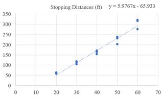
Suppose that both the explanatory variable and the response variable are speed (mph) and stopping distance (ft). The linearity of the scatter plot is too much simpler to describe. The scatter graph is built on the basis of the given data. It is very difficult to determine the linearity by seeing the scatter graph. Now check the linearity using the residual graph

  

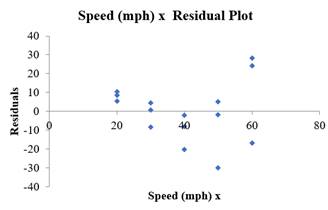
By seeing the shape of the drawn plot, there is curved pattern, which is violating the straight the sufficient condition. Therefore, the linear equation $\widehat{y}=5.9767x-65.933$ is not appropriate for the given and there is need to be re-expressed variables should be used.

(b)

To determine

To find: the re-express the data to straighten the scatter plot.

Explanation of Solution

Given:

Speed (mph)	Stopping Distances (ft)
20	64, 62, 59
30	114, 118, 105
40	153, 171, 165
50	231, 203, 238
60	317, 321, 276

Calculation:

In Part (a), it can observe that there is no linearity in the results. It is important to make it linear in order toTransform the data for the Stopping Distance response variable into a square root form. Then there's the

SQRT (Stopping Distance) appears like a new response variable.

Below, the data is mention:

Speed (mph) x	Stopping Distances (ft)	sqrt (Stopping Distances)
20	64	8
20	62	7.874007874
20	59	7.681145748
30	114	10.67707825
30	118	10.86278049
30	105	10.24695077
40	153	12.36931688
40	171	13.07669683
40	165	12.84523258
50	231	15.19868415
50	203	14.24780685
50	238	15.42724862
60	317	17.80449381
60	321	17.91647287
60	276	16.61324773

Graph:

  

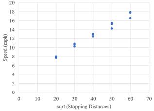
It may conclude from the scatter plot that this is a good model to fit in. it can tell from this, the square root of the distance linearizes the diagram.

(c)

To determine

To construct: the appropriate model.

Answer to Problem 15E

  $\widehat{y}=0.2355x+3.3034$

Explanation of Solution

Speed (mph)	Stopping Distances (ft)
20	64, 62, 59
30	114, 118, 105
40	153, 171, 165
50	231, 203, 238
60	317, 321, 276

Calculation:

	Coefficients	Standard Error	t Stat
Intercept	3.303404005	0.347689827	9.501008521
Speed (mph) x	0.235483506	0.008195128	28.73457391

Regression Statistics
Multiple R	0.992219418
R Square	0.984499373
Adjusted R Square	0.983307017
Standard Error	0.448865636
Observations	15

Predicted regression equation

  $\widehat{y}=0.2355x+3.3034$

(d)

To determine

To Calculate:the stopping distance for a car travelling 55 mph.

Answer to Problem 15E

263.251

Explanation of Solution

Given:

  $x=55$

Formula used:

  $\widehat{y}=\sqrt{\text{stopping}\text{distance}}=0.2355x+3.3034$

Calculation:

  $\begin{array}{c}\widehat{y}=\sqrt{\text{stopping}\text{distance}}=0.2355x+3.3034\\ =0.2355\left(55\right)+3.3034\\ =16.225\\ \text{stopping}\text{distance}={\left(16.225\right)}^2\\ =263.251\text{feet}\end{array}$

(e)

To determine

To Calculate:the stopping distance for a car travelling 70 mph.

Explanation of Solution

Given:

  $x=70$

Formula used:

  $\widehat{y}=\sqrt{\text{stopping}\text{distance}}=0.2355x+3.3034$

Calculation:

  $\begin{array}{c}\widehat{y}=\sqrt{\text{stopping}\text{distance}}=0.2355x+3.3034\\ =0.2355\left(70\right)+3.3034\\ =19.75\\ \text{stopping}\text{distance}={\left(19.75\right)}^2\\ =390.063\text{feet}\end{array}$

(f)

To determine

To find: the confidence that place in these predictions.

Explanation of Solution

The results got in part (c), the coefficient of determination is $R^2=0.9845$ and also the smallest value of s would be 0.448866 is confident.