Chapter 10, Problem 12P

To determine

if the event would cause a moment along or a shift in the position of the long run aggregate supply curve.

Concept introduction:

Aggregate Demand Curve (AD) Curve- The aggregate demand is a macro perspective of the individual demand analysis. It is a quantitative aggregate of the individual demand for goods and services in the economy. In other words, it is the total quantity of all goods and services demanded by the economy at different price levels. Like the individual demand curve, the aggregate demand curve is a downward sloping curve implying an inverse relationship between the quantity demanded and price. Graphically, the curve is drawn on a two-dimensional frame where price level is measured on Y-axis and the real quantity of the goods and services purchased as measured by the Real GDP is measured on X-axis.

Aggregate Supply Curve (AC) Curve- The aggregate supply curve is the quantity of real GDP supplied by the economy at different price levels. It is a quantitative aggregate of the quantity of goods and services supplied by the producers in the economy at varying price levels.

Short run ASC (SRAS) Curve- The relationship between the quantity of the real GDP supplied by the economy at different price levels in a period when the all factors of production are not variable and increased prices do not culminate into increased input prices, is represented by the Short Run ASC or SRAS Curve. This is a macroeconomic parallel of the individual supply analysis where higher quantity is supplied at higher prices and is graphically represented as an upward sloping curve implying a direct relationship between quantity supplied and price.

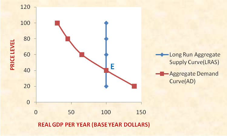
Long Run Aggregate Supply Curve (LRAS) Curve- In the long run with all factors variable, the increased price level translates into higher cost of living and higher input prices. The producers adjust the production levels to meet the increased cost of production. Thus, in the long run, the supply does not change in reaction to changes in the aggregate demand. This long run relationship between the Aggregate supply and price level is the Long Run Aggregate Supply (LRAS) Curve and is graphically represented as a straight line parallel to the Y-Axis implying perfect inelasticity of supply.

Long Run Equilibrium and the AS-AD Model- The point of intersection of the SRAS Curve, the LRAS Curve and the AD Curve is studied under the AS-AD Model and depicts the long run equilibrium in the economy.

The figure below depicts an economy in a state of long run equilibrium at Point E where LRAS curve equals the AD curve.