
Concept explainers
Videos
a.
Construct a time series plot for temperature using the given data.
Comment on the pattern of obtained time series plot.
a.
Answer to Problem 82SE
Output obtained from MINITAB is given below:
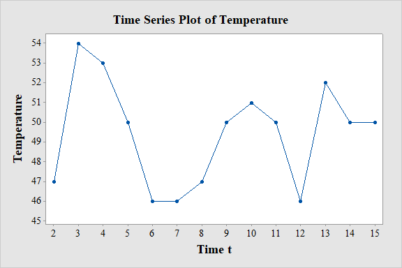
The obtained time series plot represents a cyclic pattern of temperature.
Explanation of Solution
Given info:
The data represents the observed value of response variable x at time t. The observed values are
Calculation:
Software Procedure:
Step-by-step procedure to draw the time series plot for temperature using the MINITAB software:
- Choose Graph > Time Series Plot.
- Choose Simple, and then click OK.
- In Series, enter the column of Temperature.
- Click OK.
Observation:
Time series plot shows that the highest temperature is at time 3 and the lowest temperature is at time 6 and 7. From the graph it can be concluded that temperature oscillates with the change in time. Overall the plot represents a cyclic pattern of temperature.
b.
Find the smoothed value
b.
Answer to Problem 82SE
Smoothed values
| Time t | ||
| 2 | 47 | 47 |
| 3 | 54 | 47.7 |
| 4 | 53 | 48.2 |
| 5 | 50 | 48.4 |
| 6 | 46 | 48.2 |
| 7 | 46 | 48 |
| 8 | 47 | 47.9 |
| 9 | 50 | 48.1 |
| 10 | 51 | 48.4 |
| 11 | 50 | 48.5 |
| 12 | 46 | 48.3 |
| 13 | 52 | 48.6 |
| 14 | 50 | 48.8 |
| 15 | 50 | 48.9 |
Smoothed values
| Time t | ||
| 2 | 47 | 47 |
| 3 | 54 | 50.5 |
| 4 | 53 | 51.8 |
| 5 | 50 | 50.9 |
| 6 | 46 | 48.4 |
| 7 | 46 | 47.2 |
| 8 | 47 | 47.1 |
| 9 | 50 | 48.6 |
| 10 | 51 | 49.8 |
| 11 | 50 | 49.9 |
| 12 | 46 | 47.9 |
| 13 | 52 | 50 |
| 14 | 50 | 50 |
| 15 | 50 | 50 |
Explanation of Solution
Calculation:
The exponential smoothing equation is
Smoothed values
Here, to calculate the smoothed value
That is,
Moreover, it is given that
Hence, the smoothed value
Thus, the smoothed value at time 2 is
The smoothed value
Thus, the smoothed value at time 3 is
Similarly, smoothed values for the remaining times are given below:
| Time t | ||
| 2 | 47 | 47 |
| 3 | 54 | 47.7 |
| 4 | 53 | 48.2 |
| 5 | 50 | 48.4 |
| 6 | 46 | 48.2 |
| 7 | 46 | 48 |
| 8 | 47 | 47.9 |
| 9 | 50 | 48.1 |
| 10 | 51 | 48.4 |
| 11 | 50 | 48.5 |
| 12 | 46 | 48.3 |
| 13 | 52 | 48.6 |
| 14 | 50 | 48.8 |
| 15 | 50 | 48.9 |
Smoothed values
Here, to calculate the smoothed value
That is,
Moreover, it is given that
Hence, the smoothed value
Thus, the smoothed value at time 2 is
The smoothed value
Thus, the smoothed value at time 3 is
Similarly, smoothed values for the remaining times are given below:
| Time t | ||
| 2 | 47 | 47 |
| 3 | 54 | 50.5 |
| 4 | 53 | 51.8 |
| 5 | 50 | 50.9 |
| 6 | 46 | 48.4 |
| 7 | 46 | 47.2 |
| 8 | 47 | 47.1 |
| 9 | 50 | 48.6 |
| 10 | 51 | 49.8 |
| 11 | 50 | 49.9 |
| 12 | 46 | 47.9 |
| 13 | 52 | 50 |
| 14 | 50 | 50 |
| 15 | 50 | 50 |
c.
Find the number of values of
Find the change in the coefficient of
c.
Answer to Problem 82SE
The value of
The coefficient on
Explanation of Solution
Calculation:
The exponential smoothing equation is
Substituting the value,
Substituting the value,
Continuing the same computational procedure till the value of
Now, the equation reduces as follows:
The value of
Now, the exponential smoothing equation
Here, from the above obtained equation it is seen that the value of
Here, form the equation it can be said that the coefficient of
Moreover, the smoothing constant
That is,
Hence the value of
Therefore, the coefficient on
c.
Explain the sensitivity of the initialization of
c.
Answer to Problem 82SE
The smoothed series
Explanation of Solution
Calculation:
From part (c), the exponential smoothing equation is,
The substitution of of
Here, form the equation it can be said that the coefficient of
Moreover, the smoothing constant
That is,
Hence the value of
Therefore, the smoothed series
Want to see more full solutions like this?
Chapter 1 Solutions
WEBASSIGN ACCESS FOR PROBABILITY & STATS


- The accompanying data shows the fossil fuels production, fossil fuels consumption, and total energy consumption in quadrillions of BTUs of a certain region for the years 1986 to 2015. Complete parts a and b. Develop line charts for each variable and identify the characteristics of the time series (that is, random, stationary, trend, seasonal, or cyclical). What is the line chart for the variable Fossil Fuels Production?arrow_forwardThe accompanying data shows the fossil fuels production, fossil fuels consumption, and total energy consumption in quadrillions of BTUs of a certain region for the years 1986 to 2015. Complete parts a and b. Year Fossil Fuels Production Fossil Fuels Consumption Total Energy Consumption1949 28.748 29.002 31.9821950 32.563 31.632 34.6161951 35.792 34.008 36.9741952 34.977 33.800 36.7481953 35.349 34.826 37.6641954 33.764 33.877 36.6391955 37.364 37.410 40.2081956 39.771 38.888 41.7541957 40.133 38.926 41.7871958 37.216 38.717 41.6451959 39.045 40.550 43.4661960 39.869 42.137 45.0861961 40.307 42.758 45.7381962 41.732 44.681 47.8261963 44.037 46.509 49.6441964 45.789 48.543 51.8151965 47.235 50.577 54.0151966 50.035 53.514 57.0141967 52.597 55.127 58.9051968 54.306 58.502 62.4151969 56.286…arrow_forwardFor each of the time series, construct a line chart of the data and identify the characteristics of the time series (that is, random, stationary, trend, seasonal, or cyclical). Month PercentApr 1972 4.97May 1972 5.00Jun 1972 5.04Jul 1972 5.25Aug 1972 5.27Sep 1972 5.50Oct 1972 5.73Nov 1972 5.75Dec 1972 5.79Jan 1973 6.00Feb 1973 6.02Mar 1973 6.30Apr 1973 6.61May 1973 7.01Jun 1973 7.49Jul 1973 8.30Aug 1973 9.23Sep 1973 9.86Oct 1973 9.94Nov 1973 9.75Dec 1973 9.75Jan 1974 9.73Feb 1974 9.21Mar 1974 8.85Apr 1974 10.02May 1974 11.25Jun 1974 11.54Jul 1974 11.97Aug 1974 12.00Sep 1974 12.00Oct 1974 11.68Nov 1974 10.83Dec 1974 10.50Jan 1975 10.05Feb 1975 8.96Mar 1975 7.93Apr 1975 7.50May 1975 7.40Jun 1975 7.07Jul 1975 7.15Aug 1975 7.66Sep 1975 7.88Oct 1975 7.96Nov 1975 7.53Dec 1975 7.26Jan 1976 7.00Feb 1976 6.75Mar 1976 6.75Apr 1976 6.75May 1976…arrow_forward
- Hi, I need to make sure I have drafted a thorough analysis, so please answer the following questions. Based on the data in the attached image, develop a regression model to forecast the average sales of football magazines for each of the seven home games in the upcoming season (Year 10). That is, you should construct a single regression model and use it to estimate the average demand for the seven home games in Year 10. In addition to the variables provided, you may create new variables based on these variables or based on observations of your analysis. Be sure to provide a thorough analysis of your final model (residual diagnostics) and provide assessments of its accuracy. What insights are available based on your regression model?arrow_forwardI want to make sure that I included all possible variables and observations. There is a considerable amount of data in the images below, but not all of it may be useful for your purposes. Are there variables contained in the file that you would exclude from a forecast model to determine football magazine sales in Year 10? If so, why? Are there particular observations of football magazine sales from previous years that you would exclude from your forecasting model? If so, why?arrow_forwardStat questionsarrow_forward
- 1) and let Xt is stochastic process with WSS and Rxlt t+t) 1) E (X5) = \ 1 2 Show that E (X5 = X 3 = 2 (= = =) Since X is WSSEL 2 3) find E(X5+ X3)² 4) sind E(X5+X2) J=1 ***arrow_forwardProve that 1) | RxX (T) | << = (R₁ " + R$) 2) find Laplalse trans. of Normal dis: 3) Prove thy t /Rx (z) | < | Rx (0)\ 4) show that evary algebra is algebra or not.arrow_forwardFor each of the time series, construct a line chart of the data and identify the characteristics of the time series (that is, random, stationary, trend, seasonal, or cyclical). Month Number (Thousands)Dec 1991 65.60Jan 1992 71.60Feb 1992 78.80Mar 1992 111.60Apr 1992 107.60May 1992 115.20Jun 1992 117.80Jul 1992 106.20Aug 1992 109.90Sep 1992 106.00Oct 1992 111.80Nov 1992 84.50Dec 1992 78.60Jan 1993 70.50Feb 1993 74.60Mar 1993 95.50Apr 1993 117.80May 1993 120.90Jun 1993 128.50Jul 1993 115.30Aug 1993 121.80Sep 1993 118.50Oct 1993 123.30Nov 1993 102.30Dec 1993 98.70Jan 1994 76.20Feb 1994 83.50Mar 1994 134.30Apr 1994 137.60May 1994 148.80Jun 1994 136.40Jul 1994 127.80Aug 1994 139.80Sep 1994 130.10Oct 1994 130.60Nov 1994 113.40Dec 1994 98.50Jan 1995 84.50Feb 1995 81.60Mar 1995 103.80Apr 1995 116.90May 1995 130.50Jun 1995 123.40Jul 1995 129.10Aug 1995…arrow_forward
- For each of the time series, construct a line chart of the data and identify the characteristics of the time series (that is, random, stationary, trend, seasonal, or cyclical). Year Month Units1 Nov 42,1611 Dec 44,1862 Jan 42,2272 Feb 45,4222 Mar 54,0752 Apr 50,9262 May 53,5722 Jun 54,9202 Jul 54,4492 Aug 56,0792 Sep 52,1772 Oct 50,0872 Nov 48,5132 Dec 49,2783 Jan 48,1343 Feb 54,8873 Mar 61,0643 Apr 53,3503 May 59,4673 Jun 59,3703 Jul 55,0883 Aug 59,3493 Sep 54,4723 Oct 53,164arrow_forwardHigh Cholesterol: A group of eight individuals with high cholesterol levels were given a new drug that was designed to lower cholesterol levels. Cholesterol levels, in milligrams per deciliter, were measured before and after treatment for each individual, with the following results: Individual Before 1 2 3 4 5 6 7 8 237 282 278 297 243 228 298 269 After 200 208 178 212 174 201 189 185 Part: 0/2 Part 1 of 2 (a) Construct a 99.9% confidence interval for the mean reduction in cholesterol level. Let a represent the cholesterol level before treatment minus the cholesterol level after. Use tables to find the critical value and round the answers to at least one decimal place.arrow_forwardI worked out the answers for most of this, and provided the answers in the tables that follow. But for the total cost table, I need help working out the values for 10%, 11%, and 12%. A pharmaceutical company produces the drug NasaMist from four chemicals. Today, the company must produce 1000 pounds of the drug. The three active ingredients in NasaMist are A, B, and C. By weight, at least 8% of NasaMist must consist of A, at least 4% of B, and at least 2% of C. The cost per pound of each chemical and the amount of each active ingredient in one pound of each chemical are given in the data at the bottom. It is necessary that at least 100 pounds of chemical 2 and at least 450 pounds of chemical 3 be used. a. Determine the cheapest way of producing today’s batch of NasaMist. If needed, round your answers to one decimal digit. Production plan Weight (lbs) Chemical 1 257.1 Chemical 2 100 Chemical 3 450 Chemical 4 192.9 b. Use SolverTable to see how much the percentage of…arrow_forward
 College AlgebraAlgebraISBN:9781305115545Author:James Stewart, Lothar Redlin, Saleem WatsonPublisher:Cengage Learning
 Glencoe Algebra 1, Student Edition, 9780079039897...AlgebraISBN:9780079039897Author:CarterPublisher:McGraw Hill
 Algebra and Trigonometry (MindTap Course List)AlgebraISBN:9781305071742Author:James Stewart, Lothar Redlin, Saleem WatsonPublisher:Cengage Learning
 Trigonometry (MindTap Course List)TrigonometryISBN:9781337278461Author:Ron LarsonPublisher:Cengage Learning
 Big Ideas Math A Bridge To Success Algebra 1: Stu...AlgebraISBN:9781680331141Author:HOUGHTON MIFFLIN HARCOURTPublisher:Houghton Mifflin Harcourt