via python. It’s the -number of accidents v hour of day -number of accidents v time period - relative distribution graph With these graphs are there any statistical a
via python. It’s the -number of accidents v hour of day -number of accidents v time period - relative distribution graph With these graphs are there any statistical a
A First Course in Probability (10th Edition)
10th Edition
ISBN:9780134753119
Author:Sheldon Ross
Publisher:Sheldon Ross
Chapter1: Combinatorial Analysis
Section: Chapter Questions
Problem 1.1P: a. How many different 7-place license plates are possible if the first 2 places are for letters and...
Related questions
Question
I am planning to investigate the effect of time of day on number of road accidents. i have linked the graphs I’ve currently produced via python. It’s the
-number of accidents v hour of day
-number of accidents v time period
- relative distribution graph
With these graphs are there any statistical and numerical results (e.g
![=[9]:
30-
25
8
Percentage of Accidents
8
5
0
Relative Distribution of Accidents across Time Segments
Morning (Peak)
7AM - 10AM
ah.
Late Morning Afternoon (Off-peak) school&work Evening (Off-peak)
10AM - 12PM 12PM - 2:59 PM 3PM - 7PM
Time Segments
Late Night
7PM - 11:59 PM 12AM - 4:59 AM](/v2/_next/image?url=https%3A%2F%2Fcontent.bartleby.com%2Fqna-images%2Fquestion%2F5b1635d1-e3d3-48fc-8dcf-0165292a3c5a%2F95be2dc8-c6b8-43ee-a1a5-9e376d6d98f8%2Fprkbe5r_processed.png&w=3840&q=75)
Transcribed Image Text:=[9]:
30-
25
8
Percentage of Accidents
8
5
0
Relative Distribution of Accidents across Time Segments
Morning (Peak)
7AM - 10AM
ah.
Late Morning Afternoon (Off-peak) school&work Evening (Off-peak)
10AM - 12PM 12PM - 2:59 PM 3PM - 7PM
Time Segments
Late Night
7PM - 11:59 PM 12AM - 4:59 AM
![]:
Accident Count
160000
140000
120000
100000
80000
60000
40000
20000
0
Accident Count by Hour of the Day
10.0
Hour of the Day
14.0
15.0
16.0
17.0
18.0
19.0
20.0
21.0
22.0
23.0](/v2/_next/image?url=https%3A%2F%2Fcontent.bartleby.com%2Fqna-images%2Fquestion%2F5b1635d1-e3d3-48fc-8dcf-0165292a3c5a%2F95be2dc8-c6b8-43ee-a1a5-9e376d6d98f8%2Fdwvh61p_processed.png&w=3840&q=75)
Transcribed Image Text:]:
Accident Count
160000
140000
120000
100000
80000
60000
40000
20000
0
Accident Count by Hour of the Day
10.0
Hour of the Day
14.0
15.0
16.0
17.0
18.0
19.0
20.0
21.0
22.0
23.0
Expert Solution
This question has been solved!
Explore an expertly crafted, step-by-step solution for a thorough understanding of key concepts.
Step by step
Solved in 3 steps

Follow-up Questions
Read through expert solutions to related follow-up questions below.
Follow-up Question
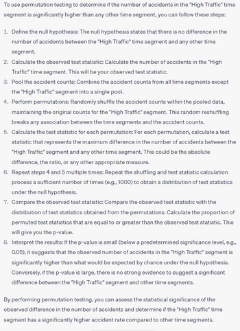
i linked an image from chatgpt that explains the steps i need to go through to determine if the number of accidents in the "High Traffic" time segment is significantly higher than any other time segment can you read it and let me know if it is the correct steps to take

Transcribed Image Text:To use permutation testing to determine if the number of accidents in the "High Traffic" time
segment is significantly higher than any other time segment, you can follow these steps:
1. Define the null hypothesis: The null hypothesis states that there is no difference in the
number of accidents between the "High Traffic" time segment and any other time
segment.
2. Calculate the observed test statistic: Calculate the number of accidents in the "High
Traffic" time segment. This will be your observed test statistic.
3. Pool the accident counts: Combine the accident counts from all time segments except
the "High Traffic" segment into a single pool.
4. Perform permutations: Randomly shuffle the accident counts within the pooled data,
maintaining the original counts for the "High Traffic" segment. This random reshuffling
breaks any association between the time segments and the accident counts.
5. Calculate the test statistic for each permutation: For each permutation, calculate a test
statistic that represents the maximum difference in the number of accidents between the
"High Traffic" segment and any other time segment. This could be the absolute
difference, the ratio, or any other appropriate measure.
6. Repeat steps 4 and 5 multiple times: Repeat the shuffling and test statistic calculation
process a sufficient number of times (e.g., 1000) to obtain a distribution of test statistics
under the null hypothesis.
7. Compare the observed test statistic: Compare the observed test statistic with the
distribution of test statistics obtained from the permutations. Calculate the proportion of
permuted test statistics that are equal to or greater than the observed test statistic. This
will give you the p-value.
8. Interpret the results: If the p-value is small (below a predetermined significance level, e.g.,
0.05), it suggests that the observed number of accidents in the "High Traffic" segment is
significantly higher than what would be expected by chance under the null hypothesis.
Conversely, if the p-value is large, there is no strong evidence to suggest a significant
difference between the "High Traffic" segment and other time segments.
By performing permutation testing, you can assess the statistical significance of the
observed difference in the number of accidents and determine if the "High Traffic" time
segment has a significantly higher accident rate compared to other time segments.
Solution
Recommended textbooks for you

A First Course in Probability (10th Edition)
Probability
ISBN:
9780134753119
Author:
Sheldon Ross
Publisher:
PEARSON


A First Course in Probability (10th Edition)
Probability
ISBN:
9780134753119
Author:
Sheldon Ross
Publisher:
PEARSON
