The mean inspection time, using the current method of quality control, has been found over a long period of time to be 160 seconds. Your manager decides to introduce a new method of quality control aimed at reducing this to as short as possible and so she expects the new method to produce a smaller mean. A random sample of measurement of inspection time taken after the new method had become established gave the following distribution:   Time (sec) 120 129 135 144 157 173 179 191 Number 1 3 2 3 4 3 3 4   Your manager thinks that the introduction of the new method of inspection has been very                                          effective in reducing the inspection time. Using the data provided and assuming the inspection time to be normally distributed with a standard deviation of 28 seconds, test this hypothesis at 5% level of significance

MATLAB: An Introduction with Applications
6th Edition
ISBN:9781119256830
Author:Amos Gilat
Publisher:Amos Gilat
Chapter1: Starting With Matlab
Section: Chapter Questions
Problem 1P
icon
Related questions
Question

The mean inspection time, using the current method of quality control, has been found over a long period of time to be 160 seconds. Your manager decides to introduce a new method of quality control aimed at reducing this to as short as possible and so she expects the new method to produce a smaller mean. A random sample of measurement of inspection time taken after the new method had become established gave the following distribution:


Time (sec)

120

129

135

144

157

173

179

191

Number

1

3

2

3

4

3

3

4


Your manager thinks that the introduction of the new method of inspection has been very                                          effective in reducing the inspection time. Using the data provided and assuming the inspection time to be normally distributed with a standard deviation of 28 seconds, test this hypothesis at 5% level of significance

Expert Solution
trending now

Trending now

This is a popular solution!

steps

Step by step

Solved in 2 steps with 1 images

Blurred answer
Follow-up Questions
Read through expert solutions to related follow-up questions below.
Follow-up Question

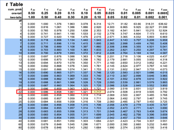
Can you explain how the highlighted boxes in the attached image a little better?

The T table i have, which is also attached( given the degree of freedom is 22)  gives a value of 1.717? 

Whereas you have given values of -1.64. Then a P value of 0.432? Can you explain further how you have reached these different figures?

2
x - l
S/√n
=
At 5% level of significance. α = 0.05
Critical value
LLAR
=
=
& P-value
159 - 160
28
P
-0.1713
20.05 =-1.64
2 <0·1213]
0.432
$ Obtained from 2-table
lor Normal probability
calculator 4
Since. 2 > 2x
and P-value > α, hence
We accept to at 5% level of significance.
|1t μ = 160.
Conclude that, new method of inspection is not
Transcribed Image Text:2 x - l S/√n = At 5% level of significance. α = 0.05 Critical value LLAR = = & P-value 159 - 160 28 P -0.1713 20.05 =-1.64 2 <0·1213] 0.432 $ Obtained from 2-table lor Normal probability calculator 4 Since. 2 > 2x and P-value > α, hence We accept to at 5% level of significance. |1t μ = 160. Conclude that, new method of inspection is not
t Table
cum. prob
one-tail
two-tails 1.00
df
1
2
3
8
9
10
11
12
13
14
15
16
17
18
19
20
21
22
23
24
25
26
1.50
0.50
27
28
0.000 1.000
0.000
0.816
1.00
1.75
0.25
0.20
0.50 0.40
0.000 0.697
0.000
0.695
0.000 0.694
0.000 0.692
1.376
1.061 1.386
0.000
0.765
0.978
1.250
0.741 0.941 1.190
0.000
0.000
0.727
0.000 0.718
0.000
0.711
0.000 0.706
0.000
0.703
0.000
0.700
0.000
0.000
0.000
0.000
0.920
0.906
1.90
0.10
0.15
0.30 0.20
1.156
1.134 1.440
0.896
1.119 1.415
0.889
1.108
1.397
0.883
1.100
1.383
0.879 1.093 1.372
1.363
1.356
0.876
0.873
0.870
0.868
1.963 3.078
1.886
1.638
2.353
1.533 2.132
1.476 2.015
1.088
1.083
1.079
1.076
1.350
1.345
0.691
0.866
1.074
0.690 0.865 1.071
0.689
0.863 1.069
0.688 0.862 1.067 1.330
0.688 0.861 1.066 1.328
0.860 1.064
0.000
0.000
0.687
1.325
0.000
0.686
0.859
1.063
1.323
0.000
0.686 0.858
1.061
1.321
0.000 0.685
0.858 1.060
1.319
0.000 0.685 0.857 1.059 1.318
0.000 0.684 0.856 1.058 1.316
0.000 0.684 0.856 1.058 1.315
0.000 0.684 0.855 1.057 1.314
1.056
1.313
0.000 0.683 0.855
0.000 0.683 0.854
29
1.055
1.311
30
1.697
0.000
0.000 0.681
1.055 1.310
1.050 1.303 1.684
40
0.683 0.854
0.851
0.848
80 0.000 0.678 0.846
60
0.000 0.679
1.296 1.671
1.045
1.043
1.292 1.664
199
1305
tas
1.375
0.05 0.025 0.01 0.005 0.001
0.10 0.05 0.02
6.314
12.71
2.920 4.303
1.341
1.337
1.333
31.82
6.965
4.541
3.747
3.365
2.571
1.943 2.447 3.143 3.707
1.895 2.365 2.998
1.860 2.306 2.896
1.833 2.262 2.821
1.812
3.182
2.776
1.796
2.201
1.782 2.179
1.771
1.729
1.725
1.721
5.208
3.499 4.785
3.355 4.501
3.250 4.297
2.228 2.764 3.169 4.144
3.106 4.025
2.718
2.681 3.055 3.930
2.160 2.650 3.012 3.852
1.761 2.145 2.624 2.977 3.787
1.753 2.131 2.602 2.947 3.733
2.583 2.921 3.686
1.746 2.120
1.740 2.110
3.646
1.734
2.567 2.898
2.878
2.539 2.861 3.579
3.610
2.528
2.845
3.552
2.518
2.831 3.527
2.508
2.819
2.500
2.807
2.101 2.552
t905
0.0005
0.01 0.002 0.001
2.093
2.086
2.080
2.074
2.069
1.717
1.714
1.711
2.064
1.708 2.060
1.706 2.056
1.703
1.701
1.699
63.66 318.31 636.62
9.925 22.327
31.599
5.841 10.215 12.924
4.604
7.173
4.032
5.893
3992
2.492
2.797
2.485 2.787
2.479 2.779
2.052 2.473 2.771
2.048 2.467
2.045 2.462 2.756
2.042
2.021
2.000
1.990
3.505
3.485
8.610
6.869
5.959
3.421
2.763 3.408
3.396
2.457 2.750 3.385
2.423 2.704
3.307
2.390
2.660
3.232
2.374 2.639 3.195
5.408
5.041
4.781
4.587
4.437
4.318
4.221
4.140
4.073
4.015
3.965
3.922
3.792
3.768
3.467 3.745
3.450
3.725
3.435
3.883
3.850
3.819
3.707
3.690
3.674
3.659
3.646
3.551
3.460
3.416
Transcribed Image Text:t Table cum. prob one-tail two-tails 1.00 df 1 2 3 8 9 10 11 12 13 14 15 16 17 18 19 20 21 22 23 24 25 26 1.50 0.50 27 28 0.000 1.000 0.000 0.816 1.00 1.75 0.25 0.20 0.50 0.40 0.000 0.697 0.000 0.695 0.000 0.694 0.000 0.692 1.376 1.061 1.386 0.000 0.765 0.978 1.250 0.741 0.941 1.190 0.000 0.000 0.727 0.000 0.718 0.000 0.711 0.000 0.706 0.000 0.703 0.000 0.700 0.000 0.000 0.000 0.000 0.920 0.906 1.90 0.10 0.15 0.30 0.20 1.156 1.134 1.440 0.896 1.119 1.415 0.889 1.108 1.397 0.883 1.100 1.383 0.879 1.093 1.372 1.363 1.356 0.876 0.873 0.870 0.868 1.963 3.078 1.886 1.638 2.353 1.533 2.132 1.476 2.015 1.088 1.083 1.079 1.076 1.350 1.345 0.691 0.866 1.074 0.690 0.865 1.071 0.689 0.863 1.069 0.688 0.862 1.067 1.330 0.688 0.861 1.066 1.328 0.860 1.064 0.000 0.000 0.687 1.325 0.000 0.686 0.859 1.063 1.323 0.000 0.686 0.858 1.061 1.321 0.000 0.685 0.858 1.060 1.319 0.000 0.685 0.857 1.059 1.318 0.000 0.684 0.856 1.058 1.316 0.000 0.684 0.856 1.058 1.315 0.000 0.684 0.855 1.057 1.314 1.056 1.313 0.000 0.683 0.855 0.000 0.683 0.854 29 1.055 1.311 30 1.697 0.000 0.000 0.681 1.055 1.310 1.050 1.303 1.684 40 0.683 0.854 0.851 0.848 80 0.000 0.678 0.846 60 0.000 0.679 1.296 1.671 1.045 1.043 1.292 1.664 199 1305 tas 1.375 0.05 0.025 0.01 0.005 0.001 0.10 0.05 0.02 6.314 12.71 2.920 4.303 1.341 1.337 1.333 31.82 6.965 4.541 3.747 3.365 2.571 1.943 2.447 3.143 3.707 1.895 2.365 2.998 1.860 2.306 2.896 1.833 2.262 2.821 1.812 3.182 2.776 1.796 2.201 1.782 2.179 1.771 1.729 1.725 1.721 5.208 3.499 4.785 3.355 4.501 3.250 4.297 2.228 2.764 3.169 4.144 3.106 4.025 2.718 2.681 3.055 3.930 2.160 2.650 3.012 3.852 1.761 2.145 2.624 2.977 3.787 1.753 2.131 2.602 2.947 3.733 2.583 2.921 3.686 1.746 2.120 1.740 2.110 3.646 1.734 2.567 2.898 2.878 2.539 2.861 3.579 3.610 2.528 2.845 3.552 2.518 2.831 3.527 2.508 2.819 2.500 2.807 2.101 2.552 t905 0.0005 0.01 0.002 0.001 2.093 2.086 2.080 2.074 2.069 1.717 1.714 1.711 2.064 1.708 2.060 1.706 2.056 1.703 1.701 1.699 63.66 318.31 636.62 9.925 22.327 31.599 5.841 10.215 12.924 4.604 7.173 4.032 5.893 3992 2.492 2.797 2.485 2.787 2.479 2.779 2.052 2.473 2.771 2.048 2.467 2.045 2.462 2.756 2.042 2.021 2.000 1.990 3.505 3.485 8.610 6.869 5.959 3.421 2.763 3.408 3.396 2.457 2.750 3.385 2.423 2.704 3.307 2.390 2.660 3.232 2.374 2.639 3.195 5.408 5.041 4.781 4.587 4.437 4.318 4.221 4.140 4.073 4.015 3.965 3.922 3.792 3.768 3.467 3.745 3.450 3.725 3.435 3.883 3.850 3.819 3.707 3.690 3.674 3.659 3.646 3.551 3.460 3.416
Solution
Bartleby Expert
SEE SOLUTION
Similar questions
  • SEE MORE QUESTIONS
Recommended textbooks for you
MATLAB: An Introduction with Applications
Statistics
ISBN:
9781119256830
Author:
Amos Gilat
Publisher:
John Wiley & Sons Inc
Probability and Statistics for Engineering and th…
Statistics
ISBN:
9781305251809
Author:
Jay L. Devore
Publisher:
Cengage Learning
Statistics for The Behavioral Sciences (MindTap C…
Statistics
ISBN:
9781305504912
Author:
Frederick J Gravetter, Larry B. Wallnau
Publisher:
Cengage Learning
Elementary Statistics: Picturing the World (7th E…
Statistics
ISBN:
9780134683416
Author:
Ron Larson, Betsy Farber
Publisher:
PEARSON
The Basic Practice of Statistics
Statistics
ISBN:
9781319042578
Author:
David S. Moore, William I. Notz, Michael A. Fligner
Publisher:
W. H. Freeman
Introduction to the Practice of Statistics
Statistics
ISBN:
9781319013387
Author:
David S. Moore, George P. McCabe, Bruce A. Craig
Publisher:
W. H. Freeman