The manager of Microsoft wants to study the # of hours per week employees spend at their desktop computers by type of industry. The manager randomly selected a sample of 5 executives from each of 3 industries studied. At the 0.05 siginificance level, can she conclude there is a difference in the mean number of hours spent per week by industry? Construction - 12, 10, 10, 12, 10 Energy - 8, 8, 6, 8, 10 Manufacturing - 10, 8, 6, 8, 10 What is the decision rule? (round 2 decimal places) (F 0.05 > ?) Complete the ANOVA Table: Source SS df MS F Treatments Error


The manager of Microsoft wants to study the # of hours per week employees spend at their desktop computers by type of industry. The manager randomly selected a sample of 5 executives from each of 3 industries studied. At the 0.05 siginificance level, can she conclude there is a difference in the
Construction - 12, 10, 10, 12, 10
Energy - 8, 8, 6, 8, 10
Manufacturing - 10, 8, 6, 8, 10
- What is the decision rule? (round 2 decimal places) (F 0.05 > ?)
- Complete the ANOVA Table:
Source SS df MS F Treatments Error

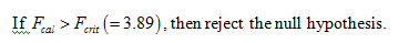
That is, there is no evidence to conclude that there is a difference in the mean number of hours spent per week by industry.

That is, there is evidence to conclude that there is a difference in the mean number of hours spent per week by industry.
Obtain the F-critical value.
Use EXCEL Procedure to obtain the F-critical value.
Follow the instruction to obtain the F-critical value.
- Open EXCEL
- Go to Data>Data Analysis.
- Choose ANOVA: Single Factor.
- Enter the input range as $A$1:$C$7.
- Select Grouped By as Columns.
- Check the Labels in the first row.
- Set the alpha as 0.05.
- Click OK.
EXCEL output:
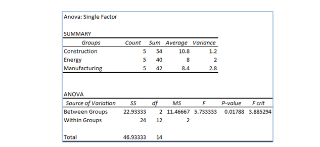
From EXCEL output, the F-critical value is 3.89
Decision rule:

Step by step
Solved in 4 steps with 6 images


