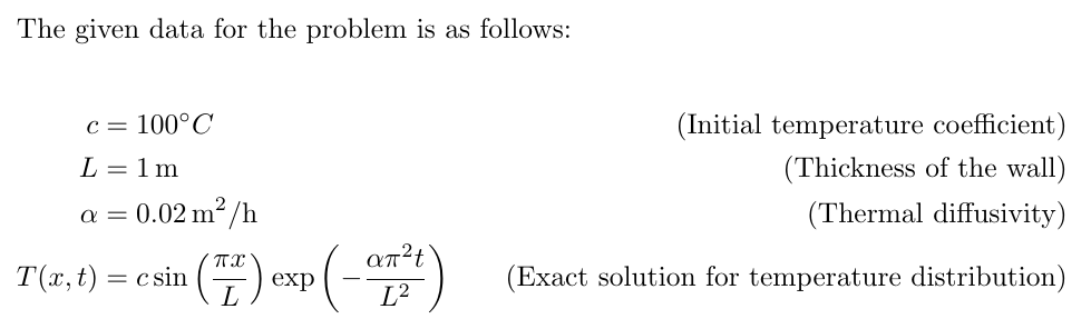
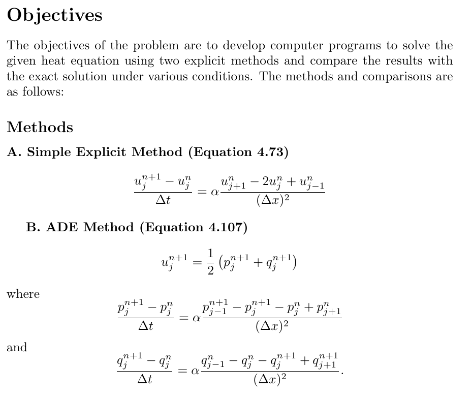
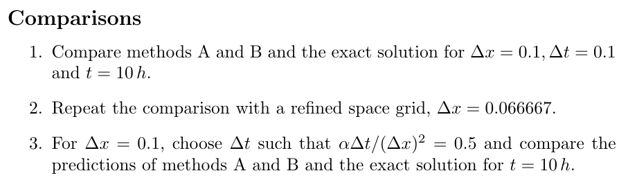
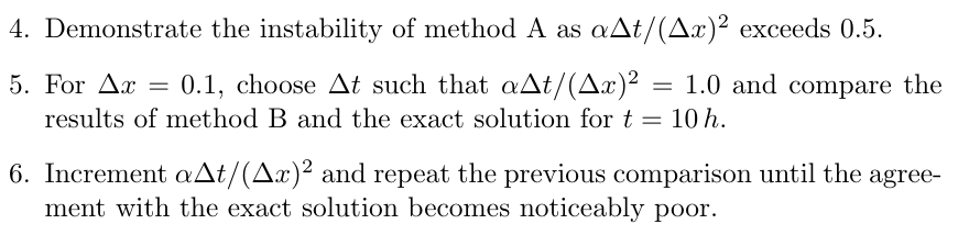
The heat equation aT at a²T ax² governs the time-dependent temperature distribution in a homogeneous constant property solid under conditions where the temperature varies only in one space dimension. Physically, this may be nearly realized in a long thin rod or very large (infinite) wall of finite thickness. Consider a large wall of thickness L whose initial temperature is given by T(t, x) = c sin îx/L. If the faces of the wall continue to be held at 0°, then a solution for the temperature at t > 0, 0≤x≤ Lis T(1.x) = cexp{- -cur²r) sin ( 7 ) n+1 For this problem, let c = 100°C, L = 1 m, a = 0.02 m²/h. We will consider two explicit methods of solution: A. Simple explicit method, Equation 4.73. Stability requires that aA/(Ax)² = for this method. B. ADE method, Equation 4.107. This particular version of the ADE method was suggested by Barakat and Clark (1966). In this algorithm, the equation for pi* can be solved explicitly starting from the boundary at x = 0, whereas the equation for q*¹ should be solved starting at the boundary at x = L. There is no stability constraint on the size of the time step for this method. Develop computer programs to solve the problem described previously by methods A and B. Also, you are to provide a capability for evaluating the exact solution for purposes of comparison. Make at least the following comparisons: 1. For Ax = 0.1, At = 0.1 [resulting in a^t/(Ax)² = 0.2], compare the results from methods A and B and the exact solution for t= 10h. A graphical comparison is suggested. 2. Repeat the aforementioned comparison after refining the space grid, that is, let Ax = 0.066667 (15 increments). Is the reduction in error as suggested by O[(Ax)2]? 3. For Ax = 0.1, choose At such that a^t/(Ax)2 = 0.5 and compare the predictions of methods A and B and the exact solution for t= 10h. 4. Demonstrate that method A does become unstable as aAt/(Ax)² exceeds 0.5. One suggestion is to plot the centerline temperature versus time for at/(Ax)²~0.6 for 10-20h of problem time. 5. For Ax = 0.1, choose At such that aAt/(Ax)² = 1.0 and compare the results of method B and the exact solution for t= 10 h. 6. Increment a^t/(Ax)² to 2, then 3, etc., and repeat comparison 5 mentioned earlier until the agreement with the exact solution becomes noticeably poor.