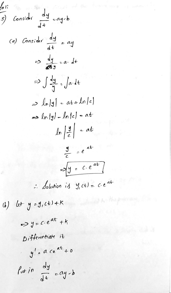
t S g Call the solution y₁ (t). b. Observe that the only difference between equations (31) and (32) is the constant -b in equation (31). Therefore, it may seem reasonable to assume that the solutions of these two equations also differ only by a constant. Test this assumption by trying to find a constant k such that y = yı(t) + k is a solution of equation (31). c. Compare your solution from part b with the solution given in the text in equation (17). Note: This method can also be used in some cases in which the constant b is replaced by a function g(t). It depends on whether you can guess the general form that the solution is likely to take. This method is described in detail in Section 3.5 in connection with second- order equations. 6. Use the method of Problem 5 to solve the equation 7. The field mouse differential equation dy -ay+b. dt population in Example 1 satisfies the = ODE dy P dt 2 - - - 450. a. Find the time at which the population becomes extinct if p(0) = 850. b. Find the time of extinction if p(0) = Po, where 0 < Po < 900. Nc. Find the initial population po if the population is to become extinct in 1 year. 8. The falling object in Example 2 satisfies the initial value