R(s) Second-order System Performance in Feedback Systems KG(s) 1+ KG(s)H(s) R(s) -K| Gc(s) = K G(s) = G(s) H(s) = 1 C(s) H(s) Ex: Sketch all the Closed Loop Roots in the S – Plane for ACLTE(S) For K Varying from Zero to Infinitive 1 (s + 1)(s + 2)(s + 4) C(s) = = 1+ K 0≤k<∞ ACLTF (S) = 1 + KG(s)H(s) T(s) = KG(s) + KG(s)H(s) ACLTF (S) = 1 + KG(s)H(s)
R(s) Second-order System Performance in Feedback Systems KG(s) 1+ KG(s)H(s) R(s) -K| Gc(s) = K G(s) = G(s) H(s) = 1 C(s) H(s) Ex: Sketch all the Closed Loop Roots in the S – Plane for ACLTE(S) For K Varying from Zero to Infinitive 1 (s + 1)(s + 2)(s + 4) C(s) = = 1+ K 0≤k<∞ ACLTF (S) = 1 + KG(s)H(s) T(s) = KG(s) + KG(s)H(s) ACLTF (S) = 1 + KG(s)H(s)

Introductory Circuit Analysis (13th Edition)
13th Edition
ISBN:9780133923605
Author:Robert L. Boylestad
Publisher:Robert L. Boylestad
Chapter1: Introduction
Section: Chapter Questions
Problem 1P: Visit your local library (at school or home) and describe the extent to which it provides literature...

Related questions
Question
This is a part of a review I'm studying, NOT a graded assignment, please do not reject. Thank you!
![**Second-order System Performance in Feedback Systems**
---
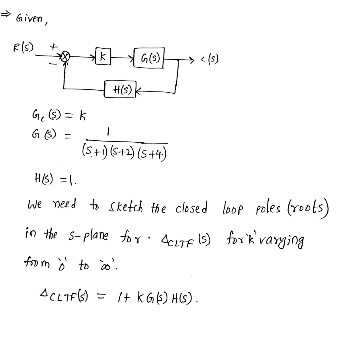
**Diagram Explanation:**
The diagram displays a block diagram of a feedback system. It consists of the following components:
- **R(s):** Input to the system.
- **K:** Gain block.
- **G(s):** Forward path transfer function.
- **H(s):** Feedback path transfer function.
- **C(s):** Output of the system, with a feedback loop from C(s) to the summing point before K.
The mathematical expression shows the transfer function for the closed-loop system:
\[ C(s) = \left[\frac{KG(s)}{1 + KG(s)H(s)}\right] R(s) \]
The gain \( K \) ranges from \( 0 \leq K < \infty \).
The characteristic equation is given by:
\[ \Delta_{CLTF}(s) = 1 + KG(s)H(s) \]
---
**Example:**
**Objective:** Sketch all the Closed Loop Roots in the S-Plane for \(\Delta_{CLTF}(s)\) for K varying from Zero to Infinite.
---
- **\( G_c(s) = K \):** Controller gain.
- **\( G(s) = \frac{1}{(s+1)(s+2)(s+4)} \):** Transfer function of the plant.
- **\( H(s) = 1 \):** Feedback transfer function.
The closed-loop transfer function is:
\[ T(s) = \frac{KG(s)}{1 + KG(s)H(s)} \]
The characteristic equation remains:
\[ \Delta_{CLTF}(s) = 1 + KG(s)H(s) \]
---
This exercise involves analyzing the roots of the characteristic equation as the gain \( K \) varies from zero to infinity, which is essential for understanding system stability and performance characteristics in control systems.](/v2/_next/image?url=https%3A%2F%2Fcontent.bartleby.com%2Fqna-images%2Fquestion%2Fecd9d238-92a1-4a47-af9e-c758e887edd1%2F67b49093-ffd8-48cd-b359-d6c8c8e56df3%2Fxcm98rp_processed.png&w=3840&q=75)
Transcribed Image Text:**Second-order System Performance in Feedback Systems**
---
**Diagram Explanation:**
The diagram displays a block diagram of a feedback system. It consists of the following components:
- **R(s):** Input to the system.
- **K:** Gain block.
- **G(s):** Forward path transfer function.
- **H(s):** Feedback path transfer function.
- **C(s):** Output of the system, with a feedback loop from C(s) to the summing point before K.
The mathematical expression shows the transfer function for the closed-loop system:
\[ C(s) = \left[\frac{KG(s)}{1 + KG(s)H(s)}\right] R(s) \]
The gain \( K \) ranges from \( 0 \leq K < \infty \).
The characteristic equation is given by:
\[ \Delta_{CLTF}(s) = 1 + KG(s)H(s) \]
---
**Example:**
**Objective:** Sketch all the Closed Loop Roots in the S-Plane for \(\Delta_{CLTF}(s)\) for K varying from Zero to Infinite.
---
- **\( G_c(s) = K \):** Controller gain.
- **\( G(s) = \frac{1}{(s+1)(s+2)(s+4)} \):** Transfer function of the plant.
- **\( H(s) = 1 \):** Feedback transfer function.
The closed-loop transfer function is:
\[ T(s) = \frac{KG(s)}{1 + KG(s)H(s)} \]
The characteristic equation remains:
\[ \Delta_{CLTF}(s) = 1 + KG(s)H(s) \]
---
This exercise involves analyzing the roots of the characteristic equation as the gain \( K \) varies from zero to infinity, which is essential for understanding system stability and performance characteristics in control systems.
Expert Solution
Step 1: State the given data.

Step by step
Solved in 7 steps with 7 images

Knowledge Booster


Learn more about
Need a deep-dive on the concept behind this application? Look no further. Learn more about this topic, electrical-engineering and related others by exploring similar questions and additional content below.Recommended textbooks for you
Introductory Circuit Analysis (13th Edition)
Electrical Engineering
ISBN:
9780133923605
Author:
Robert L. Boylestad
Publisher:
PEARSON

Delmar's Standard Textbook Of Electricity
Electrical Engineering
ISBN:
9781337900348
Author:
Stephen L. Herman
Publisher:
Cengage Learning

Programmable Logic Controllers
Electrical Engineering
ISBN:
9780073373843
Author:
Frank D. Petruzella
Publisher:
McGraw-Hill Education
Introductory Circuit Analysis (13th Edition)
Electrical Engineering
ISBN:
9780133923605
Author:
Robert L. Boylestad
Publisher:
PEARSON
Delmar's Standard Textbook Of Electricity
Electrical Engineering
ISBN:
9781337900348
Author:
Stephen L. Herman
Publisher:
Cengage Learning
Programmable Logic Controllers
Electrical Engineering
ISBN:
9780073373843
Author:
Frank D. Petruzella
Publisher:
McGraw-Hill Education

Fundamentals of Electric Circuits
Electrical Engineering
ISBN:
9780078028229
Author:
Charles K Alexander, Matthew Sadiku
Publisher:
McGraw-Hill Education

Electric Circuits. (11th Edition)
Electrical Engineering
ISBN:
9780134746968
Author:
James W. Nilsson, Susan Riedel
Publisher:
PEARSON

Engineering Electromagnetics
Electrical Engineering
ISBN:
9780078028151
Author:
Hayt, William H. (william Hart), Jr, BUCK, John A.
Publisher:
Mcgraw-hill Education,