Q"+wQ = sin wot,

Advanced Engineering Mathematics
10th Edition
ISBN:9780470458365
Author:Erwin Kreyszig
Publisher:Erwin Kreyszig
Chapter2: Second-order Linear Odes
Section: Chapter Questions
Problem 1RQ

Related questions
Question
Please do 2 I have supplied the general form of 2.27
![**2.3 Nonhomogeneous Equations**
This solution shows that the charge response is a sum of two oscillations of different frequencies. If the forcing frequency \( \omega \) is close to the natural frequency \( \omega_0 \), then the amplitude is bounded, but it is obviously large because of the factor \( \frac{1}{\omega_0^2 - \omega^2} \) occurring in the denominator. Thus the system has large oscillations when \( \omega \) is close to \( \omega_0 \).
**Example 2.27**
In the previous example, what happens if \( \omega = \omega_0 \)? Then the general solution in (2.17) is invalid because of division by zero; thus we have to re-solve the problem. The circuit equation is
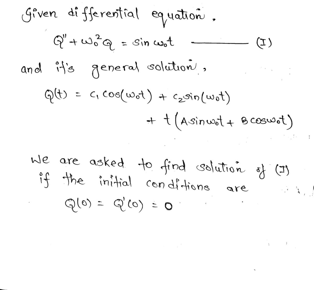
\[ Q'' + \omega_0^2 Q = \sin \omega_0 t, \tag{2.19} \]
where the circuit is forced at the same frequency as its natural frequency. The homogeneous solution is the same as before, but the particular solution now has the form
\[ Q_p(t) = t(A \sin \omega_0 t + B \cos \omega_0 t), \]
with a factor of \( t \) multiplying the terms. Therefore the general solution of (2.19) has the form
\[ Q(t) = c_1 \cos \omega_0 t + c_2 \sin \omega_0 t + t(A \sin \omega_0 t + B \cos \omega_0 t). \]
Without actually determining the constants, we can infer the nature of the response. Because of the \( t \) factor in the particular solution, the amplitude of the oscillatory response \( Q(t) \) grows in time. This is the phenomenon of *pure resonance*, or mathematical resonance. It occurs when the frequency of the external force is the same as the natural frequency of the system.
The previous example is an ideal case and physically unreasonable. All circuits have resistance, or dissipation, even though it may be small. We ask what happens if we include a small damping term in the circuit and still force it at its...](/v2/_next/image?url=https%3A%2F%2Fcontent.bartleby.com%2Fqna-images%2Fquestion%2Fc10cce41-ef51-4545-a724-9736e236d3b7%2Fa6a59dfe-e306-45ee-895f-fb67e24821b7%2Fyxzwleq_processed.jpeg&w=3840&q=75)
Transcribed Image Text:**2.3 Nonhomogeneous Equations**
This solution shows that the charge response is a sum of two oscillations of different frequencies. If the forcing frequency \( \omega \) is close to the natural frequency \( \omega_0 \), then the amplitude is bounded, but it is obviously large because of the factor \( \frac{1}{\omega_0^2 - \omega^2} \) occurring in the denominator. Thus the system has large oscillations when \( \omega \) is close to \( \omega_0 \).
**Example 2.27**
In the previous example, what happens if \( \omega = \omega_0 \)? Then the general solution in (2.17) is invalid because of division by zero; thus we have to re-solve the problem. The circuit equation is
\[ Q'' + \omega_0^2 Q = \sin \omega_0 t, \tag{2.19} \]
where the circuit is forced at the same frequency as its natural frequency. The homogeneous solution is the same as before, but the particular solution now has the form
\[ Q_p(t) = t(A \sin \omega_0 t + B \cos \omega_0 t), \]
with a factor of \( t \) multiplying the terms. Therefore the general solution of (2.19) has the form
\[ Q(t) = c_1 \cos \omega_0 t + c_2 \sin \omega_0 t + t(A \sin \omega_0 t + B \cos \omega_0 t). \]
Without actually determining the constants, we can infer the nature of the response. Because of the \( t \) factor in the particular solution, the amplitude of the oscillatory response \( Q(t) \) grows in time. This is the phenomenon of *pure resonance*, or mathematical resonance. It occurs when the frequency of the external force is the same as the natural frequency of the system.
The previous example is an ideal case and physically unreasonable. All circuits have resistance, or dissipation, even though it may be small. We ask what happens if we include a small damping term in the circuit and still force it at its...

Transcribed Image Text:**Figure 2.8**
The graph represents the plot of the solution to the differential equation \( Q'' + 0.2Q' + 2Q = \sin(\sqrt{2}t) \) with initial conditions set to zero. The system is driven at a frequency equal to the natural frequency, and there is small damping, as indicated by the gradual decrease in amplitude over time.
**EXERCISES**
1. **Plot the solution (2.18)** for several different values of \( \beta \) and \( \omega \). Include values where these two frequencies are close.
2. **Find the solution** in Example 2.27 if the initial conditions are \( Q(0) = Q'(0) = 0 \).
3. **Find the form of the general solution** of the equation \( I'' + 16I = \cos 4t \).
Expert Solution
Step 1

Step by step
Solved in 3 steps with 5 images

Recommended textbooks for you
Advanced Engineering Mathematics
Advanced Math
ISBN:
9780470458365
Author:
Erwin Kreyszig
Publisher:
Wiley, John & Sons, Incorporated

Numerical Methods for Engineers
Advanced Math
ISBN:
9780073397924
Author:
Steven C. Chapra Dr., Raymond P. Canale
Publisher:
McGraw-Hill Education

Introductory Mathematics for Engineering Applicat…
Advanced Math
ISBN:
9781118141809
Author:
Nathan Klingbeil
Publisher:
WILEY
Advanced Engineering Mathematics
Advanced Math
ISBN:
9780470458365
Author:
Erwin Kreyszig
Publisher:
Wiley, John & Sons, Incorporated
Numerical Methods for Engineers
Advanced Math
ISBN:
9780073397924
Author:
Steven C. Chapra Dr., Raymond P. Canale
Publisher:
McGraw-Hill Education
Introductory Mathematics for Engineering Applicat…
Advanced Math
ISBN:
9781118141809
Author:
Nathan Klingbeil
Publisher:
WILEY

Mathematics For Machine Technology
Advanced Math
ISBN:
9781337798310
Author:
Peterson, John.
Publisher:
Cengage Learning,

