of # o} $1 = 0.75; s2 = 0.71 E = 34.08 ; z2 = 34.32 %3D %3D n1 = 23 ; n2 = 32 %3! a. Calculate the Standard Error si,-i, = (use 3 decimal places) b. Calculate the t-test statistic using the standard error from part a. t = (use 2 decimal places) c. What are the degrees of freedom? df %3D
of # o} $1 = 0.75; s2 = 0.71 E = 34.08 ; z2 = 34.32 %3D %3D n1 = 23 ; n2 = 32 %3! a. Calculate the Standard Error si,-i, = (use 3 decimal places) b. Calculate the t-test statistic using the standard error from part a. t = (use 2 decimal places) c. What are the degrees of freedom? df %3D

MATLAB: An Introduction with Applications
6th Edition
ISBN:9781119256830
Author:Amos Gilat
Publisher:Amos Gilat
Chapter1: Starting With Matlab
Section: Chapter Questions
Problem 1P

Related questions
Question
![**Testing the Claim \( \mu_1 < \mu_2 \): A Step-by-Step Guide**
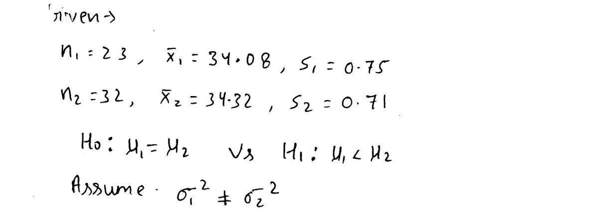
Assume the samples are normally distributed, random, and independent.
### Given Data:
\[
\sigma_1^2 \neq \sigma_2^2
\]
\( s_1 = 0.75; \, s_2 = 0.71 \)
\( \bar{x}_1 = 34.08; \, \bar{x}_2 = 34.32 \)
\( n_1 = 23; \, n_2 = 32 \)
### Steps:
**a. Calculate the Standard Error \( s_{\bar{x}_1 - \bar{x}_2} \):**
- Fill in the box (use 3 decimal places).
**b. Calculate the t-test statistic using the standard error from part a. \( t = \):**
- Fill in the box (use 2 decimal places).
**c. What are the degrees of freedom? \( df = \):**
- Fill in the box.
**d. At \( \alpha = 0.10 \). Use the distribution table to find the critical values for the rejection region. \( t_c = \):**
- Fill in the box (use 4 decimal places).
**e. Conclusion:**
What is your conclusion?
- Reject the null hypothesis and support the claim
- Accept the alternative hypothesis and reject the claim
- Accept the null hypothesis and support the claim
- Fail to reject the null hypothesis and do not support the claim
- Reject the alternative hypothesis and support the claim
Follow these steps to solve the hypothesis test and make an appropriate conclusion based on the statistical evidence.](/v2/_next/image?url=https%3A%2F%2Fcontent.bartleby.com%2Fqna-images%2Fquestion%2Fa86a1608-4622-4bb5-9da8-5fb01306e299%2F76167858-aab7-491b-9083-52cab5355bdd%2Fyhgqsc6_processed.jpeg&w=3840&q=75)
Transcribed Image Text:**Testing the Claim \( \mu_1 < \mu_2 \): A Step-by-Step Guide**
Assume the samples are normally distributed, random, and independent.
### Given Data:
\[
\sigma_1^2 \neq \sigma_2^2
\]
\( s_1 = 0.75; \, s_2 = 0.71 \)
\( \bar{x}_1 = 34.08; \, \bar{x}_2 = 34.32 \)
\( n_1 = 23; \, n_2 = 32 \)
### Steps:
**a. Calculate the Standard Error \( s_{\bar{x}_1 - \bar{x}_2} \):**
- Fill in the box (use 3 decimal places).
**b. Calculate the t-test statistic using the standard error from part a. \( t = \):**
- Fill in the box (use 2 decimal places).
**c. What are the degrees of freedom? \( df = \):**
- Fill in the box.
**d. At \( \alpha = 0.10 \). Use the distribution table to find the critical values for the rejection region. \( t_c = \):**
- Fill in the box (use 4 decimal places).
**e. Conclusion:**
What is your conclusion?
- Reject the null hypothesis and support the claim
- Accept the alternative hypothesis and reject the claim
- Accept the null hypothesis and support the claim
- Fail to reject the null hypothesis and do not support the claim
- Reject the alternative hypothesis and support the claim
Follow these steps to solve the hypothesis test and make an appropriate conclusion based on the statistical evidence.
Expert Solution
Step 1
Note: According to bartleby experts question answers guidelines an expert can solve only first three sub parts of one question rest can be reposted..

Step by step
Solved in 2 steps with 2 images

Recommended textbooks for you
MATLAB: An Introduction with Applications
Statistics
ISBN:
9781119256830
Author:
Amos Gilat
Publisher:
John Wiley & Sons Inc

Probability and Statistics for Engineering and th…
Statistics
ISBN:
9781305251809
Author:
Jay L. Devore
Publisher:
Cengage Learning

Statistics for The Behavioral Sciences (MindTap C…
Statistics
ISBN:
9781305504912
Author:
Frederick J Gravetter, Larry B. Wallnau
Publisher:
Cengage Learning
MATLAB: An Introduction with Applications
Statistics
ISBN:
9781119256830
Author:
Amos Gilat
Publisher:
John Wiley & Sons Inc
Probability and Statistics for Engineering and th…
Statistics
ISBN:
9781305251809
Author:
Jay L. Devore
Publisher:
Cengage Learning
Statistics for The Behavioral Sciences (MindTap C…
Statistics
ISBN:
9781305504912
Author:
Frederick J Gravetter, Larry B. Wallnau
Publisher:
Cengage Learning

Elementary Statistics: Picturing the World (7th E…
Statistics
ISBN:
9780134683416
Author:
Ron Larson, Betsy Farber
Publisher:
PEARSON

The Basic Practice of Statistics
Statistics
ISBN:
9781319042578
Author:
David S. Moore, William I. Notz, Michael A. Fligner
Publisher:
W. H. Freeman

Introduction to the Practice of Statistics
Statistics
ISBN:
9781319013387
Author:
David S. Moore, George P. McCabe, Bruce A. Craig
Publisher:
W. H. Freeman